Introduction to Gaussian Process Regression

Gaussian processes are a robust and flexible method in machine learning, capable of leveraging prior information to make predictions. Their primary use is in regression, where they model data by fitting. However, their utility goes beyond regression, extending to tasks like classification and clustering. When faced with training data, countless functions can potentially describe it. Gaussian processes tackle this challenge by assigning a likelihood to each function, with the average of this distribution serving as the most plausible representation of the data. Moreover, their probabilistic framework naturally incorporates prediction uncertainty, providing insights into the confidence of the results.

Introductory concepts

Gaussian processes are built upon the mathematical framework of the multivariate Gaussian distribution, which extends the familiar Gaussian (or normal) distribution to multiple random variables that are jointly normally distributed. This distribution is characterized by two key components: a mean vector, $\mu$ , and a covariance matrix, $\Sigma = \text{Cov}(X_i, X_j)$ , which describes the relationships between pairs of variables. Before diving into these concepts, we will first cover some fundamental terms from probability theory to ensure we have a shared understanding.

Generally, a multivariate Gaussian distribution is expressed as:

X = \begin{bmatrix} X_1 \\ X_2 \\ \vdots \\ X_n \end{bmatrix} \sim \mathcal{N}(\mu, \Sigma)

where $X$ is a vector of random variables.

The covariance matrix $\Sigma$ determines the shape of the distribution and, in the 2D case, can be represented as:

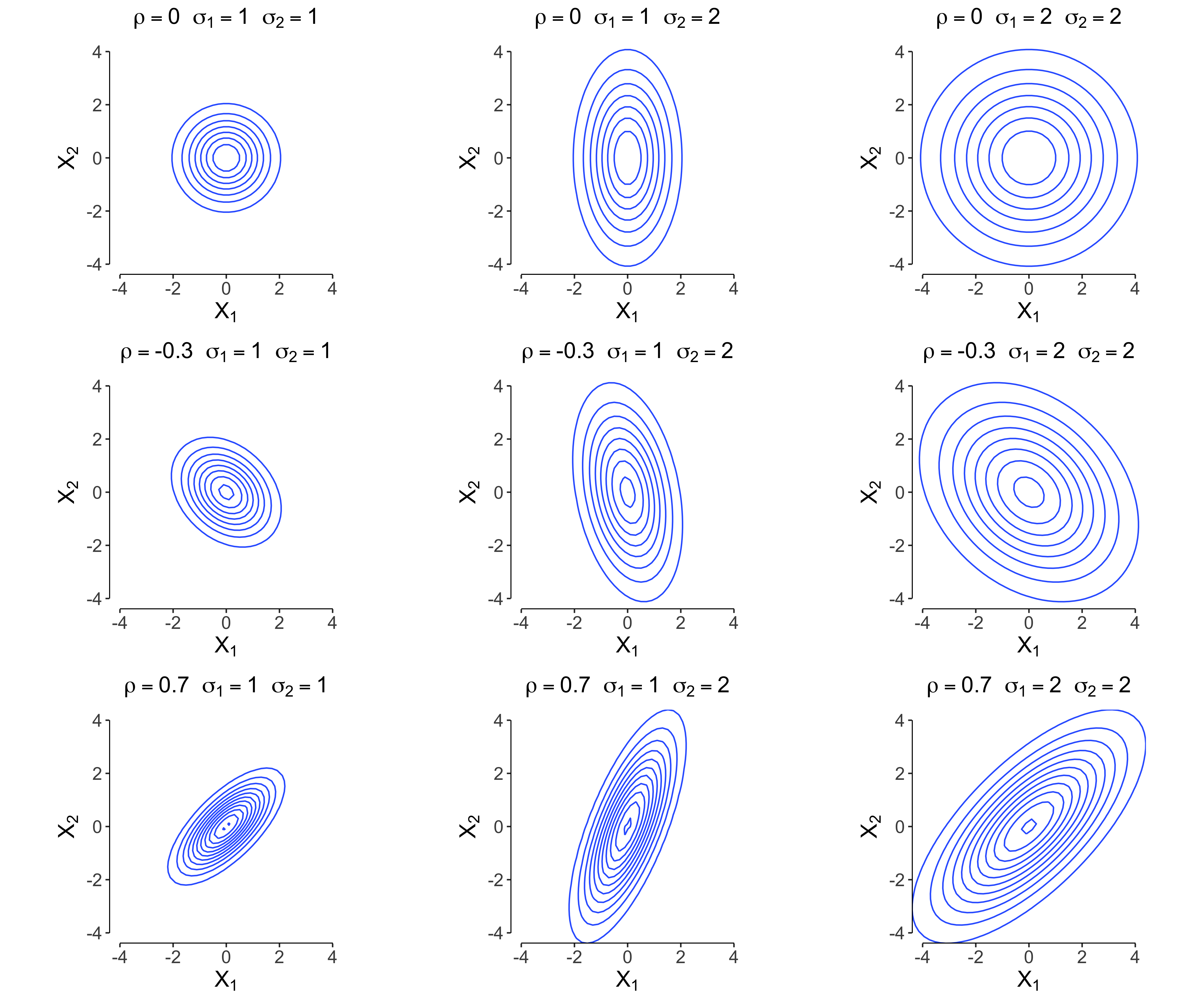
\Sigma = \begin{bmatrix} \sigma_1^2 & \sigma_1 \sigma_2 \\ \sigma_2 \sigma_1 & \sigma_2^2 \end{bmatrix}

Contour plots of the multivariate Gaussian distribution illustrate how $\Sigma$ affects the spread and orientation of the distribution. An example of such plots for different covariance matrices $\Sigma$ is shown in the figure below, demonstrating how the covariance influences the relationships between variables.

Conditioning

Suppose a joint dristribution of two vectors of gaussian random variables $X$ and $Y$

P_{X,Y} = \begin{bmatrix} X \\ Y \end{bmatrix} \sim \mathcal{N}(\mu, \Sigma) = \mathcal{N}\left( \begin{bmatrix} \mu_X \\ \mu_Y \end{bmatrix}, \begin{bmatrix} \Sigma_{XX} & \Sigma_{XY} \\ \Sigma_{YX} & \Sigma_{YY} \end{bmatrix} \right).

The covariance matrices, such as $\Sigma_{XX}$ , are themselves matrices, ensuring that the final covariance matrix has a size of $|X| + |Y|$ . We can derive the conditional multivariate distributions using the following expressions:

P_{X \mid Y} \sim \mathcal{N}\left( \mu_X + \Sigma_{XY} \Sigma_{YY}^{-1} (Y - \mu_Y), \Sigma_{XX} - \Sigma_{XY} \Sigma_{YY}^{-1} \Sigma_{YX} \right)

P_{Y \mid X} \sim \mathcal{N}\left( \mu_Y + \Sigma_{YX} \Sigma_{XX}^{-1} (X - \mu_X), \Sigma_{YY} - \Sigma_{YX} \Sigma_{XX}^{-1} \Sigma_{XY} \right).

Marginalization

Another important concept is marginalization. Marginalization over a random variable in a joint distribution involves summing (or integrating) over all possible values of the other variable in the conditional distribution.

For example, given two vectors of Gaussian random variables:

X \sim \mathcal{N}(\mu_X, \Sigma_{XX})\\ Y \sim \mathcal{N}(\mu_Y, \Sigma_{YY})

and their joint distribution $P_{X,Y}$ , we can marginalize over $Y$ as follows:

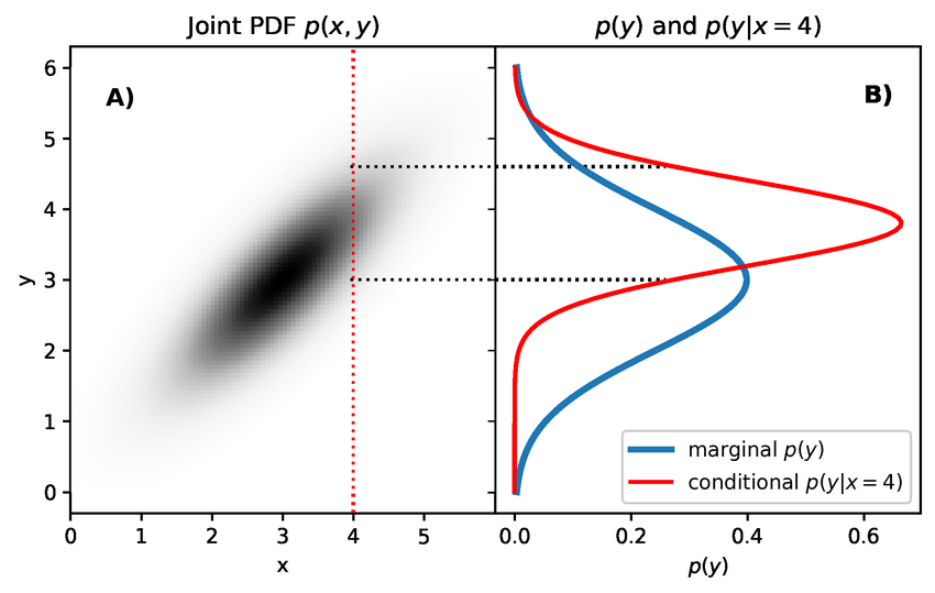
p_X(x) = \int_y p_{X,Y}(x, y) \, dy = \int_y p_{X \mid Y}(x \mid y) p_Y(y) \, dy

We can observe the differences between conditioning and marginalization in the figure below.

As shown, conditioning involves slicing through the distribution at a specific value, resulting in a distribution with one less dimension. In this case, it becomes a 1D distribution, which is a simple normal distribution. Marginalization on the other hand acts like projecting the whole 2D distribution into one dimension, in this case $Y$ .

Gaussian processes

Now that we have covered the basic concepts, we can discuss how to use them to formulate the ideas behind Gaussian processes and Gaussian process regression. The basic idea is as follows: given a set of sample positions $\{x_i\}_1^n$ of a function $f$ , we aim to determine $X_i = f(x_i)$ , where $X_i$ is the i-th entry of a random vector $X$ . This vector follows a multivariate normal distribution, meaning:

X \sim \mathcal{N}(\mu_X, \Sigma_{XX}).

For simplicity, we often assume $\mu_X = 0$ . However, calculating $\Sigma_{XX}$ involves another mathematical concept called a kernel function.

The kernel function $k$ , defined as $k \colon \mathbb{R}^n \times \mathbb{R}^n \to \mathbb{R}$ , is a measure of similarity between its inputs. A high output value for $k$ indicates high similarity between inputs, and vice versa.

In our case, the kernel function is used to compute the covariance matrix $\Sigma_{XX}$ of the multivariate normal distribution. To calculate each entry of $\text{Cov}(X, X)$ , we assume:

\text{Cov}(X_i, X_j) = k(x_i, x_j),

meaning that the covariance between two function values $X_i$ and $X_j$ is high when their corresponding inputs $x_i$ and $x_j$ are close together.

Common Kernel Functions

Below are some commonly used kernel functions in the context of Gaussian processes, some of them take hyperparameters like $l$ or $\sigma$ :

RBF Kernel:

k(t, t') = \sigma^2 \exp\left(-\frac{\|t - t'\|^2}{2l^2}\right)

Periodic Kernel:

k(t, t') = \sigma^2 \exp\left(-\frac{2 \sin^2\left(\pi \frac{|t - t'|}{p}\right)}{l^2}\right)

Linear Kernel:

k(t, t') = \sigma_b^2 + \sigma^2 (t - c)(t' - c)

Different values for hyperparameters make the similarity measure of the kernels more or less strict, leading to sharper or smoother functions in the process.

Now that we have a method to compute the covariance matrix $\Sigma_{XX}$ , we can sample a random function $f$ by drawing a sample $X$ from the multivariate normal distribution $\mathcal{N}(\mu_X, \Sigma_{XX})$ . Each entry $X_i$ in the sampled vector corresponds to the value of $f$ at $x_i$ , meaning $X_i = f(x_i).$

Gaussian Processes for Regression

We have now covered the fundamentals of Gaussian processes. Next, we will extend our understanding to explore how Gaussian processes can be applied to solve regression tasks.

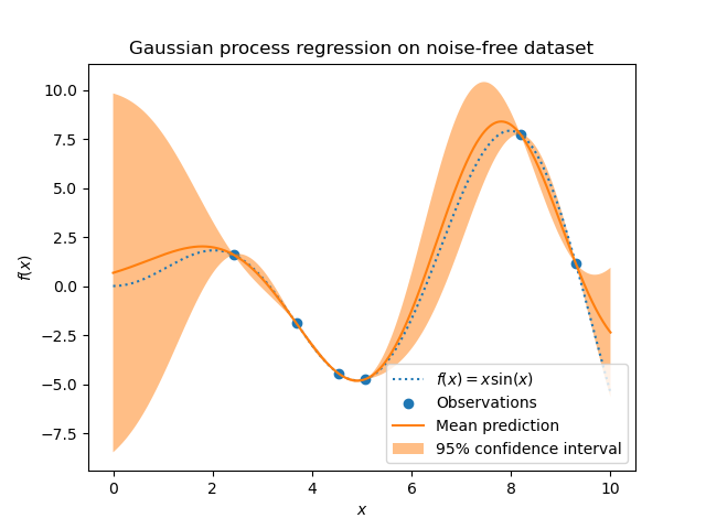
Before diving into the technical details, our objective is clear: to model a distribution of functions that pass through our training points (as shown in the image above) and are therefore able to explain the distribution of our data.

Now, let $X$ represent our test points and $Y$ our training points. We aim to model the posterior distribution $X \mid Y$ , which answers the question:

"What possible values for $X$ are there, given the training points in $Y$ ?"

This is where conditioning comes into play. Computing the distribution $P_{X|Y}$ provides us with functions $f$ that pass precisely through the points in $Y$ . Conceptually, we can think of this as slicing through a $|X| + |Y|$ -dimensional normal distribution, fixing the values at $|Y|$ locations as constants. This results in a $|X|$ -dimensional normal distribution.

As we know it is easy to calculate distribution for $P_{X, Y}$ with

P_{X,Y} \sim \mathcal{N}\left( \begin{bmatrix} \mu_X \\ \mu_Y \end{bmatrix}, \begin{bmatrix} \Sigma_{XX} & \Sigma_{XY} \\ \Sigma_{YX} & \Sigma_{YY} \end{bmatrix} \right).

From our prerequisites, we know that $P_{X|Y}$ can be calculated as:

P_{X|Y} \sim \mathcal{N}\left( \mu_X + \Sigma_{XY} \Sigma_{YY}^{-1} (Y - \mu_Y), \Sigma_{XX} - \Sigma_{XY} \Sigma_{YY}^{-1} \Sigma_{YX} \right)

This is the final distribution from which we can sample. It provides functions that pass through all points in $Y$ and whose behavior for $X$ is modeled by $P_{X|Y}$ (see image above). The figure also illustrates the 95% confidence interval ( $2\sigma$ ) and the mean function. In practice, the mean function is often the most useful for regression or prediction tasks, as it provides the expected value of the output based on the given data. Getting the mean function as well as the $2\sigma$ confidence interval is really easy once we obtained the $\mu$ and $\Sigma$ for $P_{X|Y}$ . We can just query them at the i-th point and get the respective $\mu_i$ and $\Sigma_{ii} = \sigma_i$ . This wil result in

[\mu_{X|Y}]_i = [\mu_X + \Sigma_{XY} \Sigma_{YY}^{-1} (Y - \mu_Y)]_i = [\Sigma_{XY} \Sigma_{YY}^{-1} Y]_i,

where the second equality stems from the fact that we assume $\mu_{X} = 0$ and $\mu_{Y}=0$ . For the standart deviation we get

\sigma_i = [\Sigma_{XX} - \Sigma_{XY} \Sigma_{YY}^{-1} \Sigma_{YX}. ]_{ii}

Doing this for every point $x_i$ will result in the same figure we saw above.

So in summary, gaussian processes are a flexible framework for regression, where functions are modeled as samples from a multivariate normal distribution. A kernel function is used to compute the covariance matrix $\Sigma_{XX}$ , which encodes the similarity between inputs. The posterior distribution $P_{X|Y}$ then allows us to generate functions that pass through the training points $Y$ while predicting the behavior for test points $X$ . In the end, we use the mean function provided by this posterior because it represents the most likely prediction for the underlying function.