- Published on
Introduction to Transformers - Part 00 - Architecture
- Authors

- Name
- Jan Hardtke
Transformers have revolutionized the field of natural language processing (NLP), becoming the foundation for state-of-the-art models like BERT, GPT, and T5. Introduced in the seminal paper Attention Is All You Need, transformers replaced recurrent and convolutional architectures by leveraging a novel mechanism called self-attention.
At their core, transformers process entire input sequences simultaneously, allowing them to capture global relationships within the data efficiently. This architecture not only improves performance on complex NLP tasks like machine translation and text summarization but also scales effectively to massive datasets and models.
In this series, we will explore the key components of the transformer architecture, starting with its foundational building blocks and how they enable efficient learning from sequential data.
Architecture Overview
Before explaining every bit of the transformer model in detail, we will take a quick step back and give a small Overview of the steps we will cover. The below image describes the whole model very accuarctly.
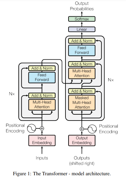
Image source
As the original transformer was designed as a sequence-to-sequence processing model, its primary application in the original paper was for translation tasks. The model takes two input sequences: a source sequence and a target sequence. While modern large language models (LLMs) have adapted and expanded upon this architecture for various tasks, we will focus for now on the original application of translation to understand the foundational principles. Later, we will explore how these principles are adjusted to form the backbone of modern LLMs.
We can see that this model takes two inputs. One for the encoder, the other for the decoder. Before feeding this inputs into the model we create tokenizations and then embeddings for each token. These embeddings are concatenated with what one calls positional encoding. As we will see later, the positional encoding gives the model a sense of ordering inside of the token sequence.
After the inputs are embedded and positional encoding is added, they are fed into the model. In the encoder, the inputs are duplicated three times and passed through a Multi-Head Attention block. Simply put, this block calculates the relative importance of each token (or its embedding) in relation to the others in the sequence. This mechanism, known as self-attention, was the groundbreaking innovation that paved the way for the development of modern large language models (LLMs).
Following the attention block, the outputs are normalized using a LayerNorm to ensure they have a mean of zero. This normalization step enhances stability and convergence during training.
Once normalized, the outputs are passed into an MLP (Multi-Layer Perceptron), which is a simple feed-forward neural network. The MLP applies additional transformations to the data, further refining the representations.
These processed outputs are then passed to another encoder block, and this process is repeated for a total of such blocks. The stacking of these blocks allows the model to capture increasingly complex patterns and relationships in the data. The decoder block in a Transformer is composed of several key components, each designed to process the target sequence and incorporate context from the input sequence encoded by the encoder.
The process begins with a masked multi-head self-attention layer. This layer operates on the embedded tokens of the target sequence and applies a mask to ensure causality. Masking ensures that each token can only attend to itself and tokens that came before it, preventing the decoder from accessing information about future tokens during sequence generation. This mechanism is crucial for autoregressive tasks like language generation, where the model predicts one token at a time.
The output of this masked self-attention, also called causal self-attention, layer is then passed into a second attention block. This second block is different from the first because it performs cross-attention. Instead of attending solely to the target sequence, it uses the outputs of the encoder for two of its inputs: the keys and values . The queries , however, are derived from the output of the masked self-attention layer. This setup allows the decoder to focus on relevant parts of the input sequence, using the context provided by the encoder's output. Importantly, this attention block is not masked, as it operates on the encoder outputs, which remain static and do not require causality constraints. Finally, the output of the cross-attention block is passed through a feed-forward neural network, similar to the one used in the encoder. This feed-forward step refines the representation and prepares it for either the next decoder layer or the output layer, where probabilities over the vocabulary are computed.
Now, this provides a high-level and simplified overview of the Transformer architecture, which gave us a foundational understanding of how this model operates. Now, let’s dive into each step of the architecture with great detail so we can implement the Transformer from scratch in our machine learning library of choice. For me, that's PyTorch.
Tokenization & Embedding
Before a language model can operate on any kind of natural language, the text needs to be transformed into a form that a computer can understand. In the field of Natural Language Processing (NLP), this process is known as tokenization.
Tokenization refers to the process of assigning a unique number (or token ID) to a unit of text. These units are typically referred to as tokens, and their definition can vary depending on the type of tokenizer used. However, in most cases, tokens are larger than a single character but smaller than an entire word.
For example:
- The word "unbelievable" might be split into sub-tokens:
"un","believe", and"able". - These sub-tokens are then mapped to unique numerical IDs.
Take the sentence The dog jumped over the green door! for example. The tokenizer of OpenAI for their GPT4o model, would make

out of this. The respective token IDs would be [976, 6446, 48704, 1072, 290, 8851, 42166, 13]. Now that we have the token IDs, the next step is to map them into a high-dimensional vector space. This is done by using the token IDs as indices into an embedding matrix, which is essentially an array of vectors. The dimension of these vectors is referred to as , often called the embedding dimension.
Positional encoding
In a Transformer, there is no inherent notion of sequence order because the architecture processes tokens in parallel. To address this, we use positional encoding, which injects information about the position of each token in the sequence into its embedding. This is achieved by adding a positional vector to the token embedding, where each position is represented using a combination of sine and cosine functions of different frequencies. These encodings allow the model to understand the relative and absolute positions of tokens within the sequence, enabling it to capture sequential information without explicit recurrence.
Mathematically, the positional encoding for a position and dimension is defined as:
To see how this works in practice, let's again consider the following sequence of tokens: [976, 6446, 48704, 1072, 290, 8851, 42166, 13]. For simplicity, we'll assume that . This means each token will be represented by a 4-dimensional embedding vector. A matrix where each row corresponds to the -dimensional embedding of a token could look like this:
import torch

# Example embedding matrix
embedding_matrix = torch.tensor([
    [0.12, 0.32, -0.54, 0.87],  # Embedding for token 976
    [0.05, 0.73, -0.12, 0.45],  # Embedding for token 6446
    [0.93, -0.34, 0.17, -0.87], # Embedding for token 48704
    [0.15, 0.22, -0.11, 0.34],  # Embedding for token 1072
    [0.29, -0.12, 0.54, -0.23], # Embedding for token 290
    [0.43, 0.56, -0.32, 0.12],  # Embedding for token 8851
    [0.91, -0.13, 0.38, -0.44], # Embedding for token 42166
    [0.07, 0.41, -0.25, 0.89]   # Embedding for token 13
])
We will then iterate through every position of the sequence and denote the current position as . For each position, we calculate the positional encoding vector and add it to the corresponding token embedding. The calculation depends on whether the dimension index is even or odd.
For an even dimension index , the positional encoding is calculated using , otherwise . The resulting positional encoding is then added element-wise to the embedding vector of the token at position . This ensures that the embedding incorporates both semantic information (from the token embeddings) and positional information (from the positional encodings).
Encoder
Now that we have the positional encoded embeddings of the source sequence, we can start feeding them into the encoder block. The first block of the encoder is the attention layer, which is not only the starting point but also the most important layer in the entire Transformer architecture.
Self-Attention
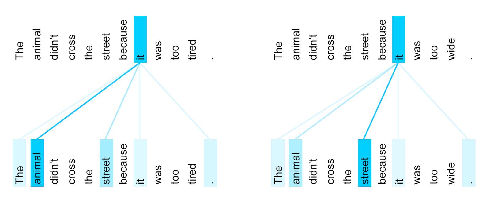
Image source
The most important concept to understand in the Transformer architecture is the so-called self-attention mechanism. This mechanism establishes an "attendance" between tokens that are likely related to each other. It helps the model understand dependencies and relationships across a sequence of tokens.
Suppose we have a sequence of tokens of length , and each token is represented by an embedding of size . This gives us a matrix of shape , where each row corresponds to the embedding of a token in the sequence.
To perform self-attention, we copy this matrix three times and create three different matrices:
- Queries ()
- Keys ()
- Values ()
Mathematically, these are obtained by multiplying the original matrix (the token embeddings), of shape , with learned weight matrices:
The self-attention mechanism computes the relationship between tokens in a sequence using Queries ( ), Keys (), and Values (). The formula for self-attention is as follows:
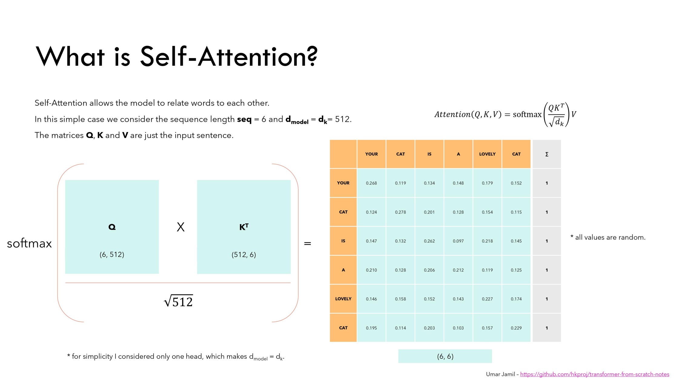
Image source
The first step in the attention mechanism is the matrix multiplication , which computes the relationships between query and key tokens.
Each row in the resulting matrix contains the dot product of the embedding of the -th token (from ) with the embeddings of all other tokens (from ). For example, the first row represents how the token "Your" relates to all other tokens in the sequence based on their embeddings.
After this, a row-wise softmax operation is applied. This converts the raw dot product scores into probabilities:
- Each value in a row is normalized to fall between and .
- The values in each row sum to , allowing us to interpret them as probabilities or percentages showing how much a query token attends to each key token.
To prevent large values from destabilizing the softmax function, the result of is divided by . This scaling is necessary because:
- The variance of the dot product increases with , leading to a standard deviation of , where is the standard deviation of and .
- Dividing by ensures that the standard deviation of the scaled values remains consistent, stabilizing the softmax operation and improving training stability.
Once we have calculated the attention weights, which form a matrix of shape , the next step is to multiply this matrix with . The matrix, which represents the values, is of shape .
The result of this multiplication is a new matrix of shape , where each row corresponds to a weighted combination of the embedding vectors, determined by the attention weights.
To understand this in detail, consider an example:
- The entry (first row, first column) of the resulting matrix is computed as the weighted sum of the first entries of all embedding vectors (rows in ), where the weights are the attention values from the first token to all other tokens.
- More generally, for an entry of the resulting matrix:
- We accumulate all -values (columns) of the embedding vectors, weighted by how much attention token pays to all other tokens.
Now intuitively:
- Each resulting row represents a "mix" of embedding vector values, where the mix is determined by the attention weights.
- The attention mechanism essentially highlights the most important parts of the embedding vectors for each token, allowing the model to focus on relevant context within the sequence.
This step combines the relationships (from the attention weights) with the actual content of the embedding vectors, producing an output that captures both context and meaning.
Skip connections & Normalization
After the self-attention layer, we end up with a matrix of shape . The next step is to add the input of the attention layer to its output, a process known as a skip connection (or residual connection).
Skip connections are introduced to address the vanishing gradient problem. During backpropagation, gradients are repeatedly multiplied as they propagate backward through the network. If the gradient values are less than 1, this repeated multiplication can lead to extremely small gradient values, effectively stalling learning in earlier layers. Adding a skip connection introduces an additive term that ensures the flow of gradients is not entirely dependent on the transformations within the layer. This mechanism helps preserve information from earlier layers and keep the gradient from underflowing during traing
This result is then passed to a normalization layer (commonly layer normalization) to ensure a mean of and unit standart deviation.
FFN
Now the last part of the encoder is a final feed-forward network. This layer applies a fully connected transformation to each token independently, enhancing the model's capacity to learn complex representations. Like the attention layer, the feed-forward network is followed by another skip connection and subsequent normalization. The output of each encoder layer has a shape of . These outputs are then passed to the decoder in the so-called cross-attention layer, which we will explore next.
Decoder
Now that we explored how the encoder transforms our input, we will look at the decoder and how we can use it the solve our task of translation. Now that we have explored how the encoder transforms the input, let’s turn our attention to the decoder and see how it helps solve the task of translation. To revisit our original goal, we are working on a translation task, where we have a source sentence in one language and a corresponding target sentence in another.
For example, consider the source sentence:The dog jumped over the green door!
Its translation in German would be:Der Hund springt über die grüne Tür!
After tokenization, these sentences are converted into sequences of token IDs. For instance:
- Source sentence (in English):
src = [976, 6446, 48704, 1072, 290, 8851, 42166, 13] - Target sentence (in German):
trg = [0, 12, 4433, 2304, 8872, 2240, 456, 2349, 13]
Here acts as a special <START> token that signifies the start of the sentence. Now the decoder will use the target (trg) sequence as input and attempt to output a sequence that is shifted by one token to the left. This means the model predicts the next token in the sequence based on the previous tokens it has seen.
For example, given the target sequence:trg = [0, 12, 4433, 2304, 8872, 2240, 456, 2349, 13]
The ground truth for the decoder will be:ground_truth = [12, 4433, 2304, 8872, 2240, 456, 2349, 13, 99999]
Here, acts as a special <END> token that signifies the end of the sequence. The decoder learns to predict this <END> token to indicate that the translation process is complete. Each token in the ground_truth corresponds to what the decoder should produce for the respective input token in the shifted target sequence.
Masked Multi-Head Attention
Now that we understand what kind of inputs (targets) are fed into the decoder, let’s examine the first block, which is called the Masked Multi-Head Attention layer. Before diving into the Multi-Head aspect, let’s briefly explore the concept of masking.
Masking
Masking refers to the process of nullifying some of the attention weights in the attention layer. This ensures that, in this block, a given token can only attend to tokens that came before it in the sequence (or itself). The purpose of masking is to enforce causality, meaning the model is not allowed to "look ahead" at future tokens while generating its output. This behavior mirrors the way the Transformer is used during sampling after it has been trained. For example, when generating text, the model predicts the next token one step at a time, based only on the tokens it has already seen. Training the model with this restriction ensures that it doesn't rely on information from tokens that are "in the future" relative to the current step. By applying masking in the attention mechanism, the Transformer learns to predict tokens in a sequential, autoregressive manner, maintaining the same causal relationship as during inference. This type of self-attention is therefore called causal self-attention. To build the mask, we use an upper triangular mask, where 1 indicates masked positions, and 0 indicates unmasked positions.
import torch

# Sequence length
seq_len = 8

# Explicitly define the upper triangular mask as a tensor
upper_triangular_mask = torch.tensor([
    [0, 1, 1, 1, 1, 1, 1, 1],
    [0, 0, 1, 1, 1, 1, 1, 1],
    [0, 0, 0, 1, 1, 1, 1, 1],
    [0, 0, 0, 0, 1, 1, 1, 1],
    [0, 0, 0, 0, 0, 1, 1, 1],
    [0, 0, 0, 0, 0, 0, 1, 1],
    [0, 0, 0, 0, 0, 0, 0, 1],
    [0, 0, 0, 0, 0, 0, 0, 0],
], dtype=torch.float32)

# Example attention scores (random values)
attention_scores = torch.randn((seq_len, seq_len))

# Apply the mask using torch.where
masked_attention_scores = torch.where(upper_triangular_mask.bool(), float('-inf'), attention_scores)
Instead of directly multiplying the attention matrices by this mask, we modify the attention mechanism by setting specific attention values to negative infinity (-inf).
Given the output of , which is of shape , we set attention values where to . This ensures that, when we apply the softmax function, these masked values are transformed to , while the other attention weights in each row still sum to .
Multi-Head Attention
Now that we have an understanding of the self-attention mechanism, let’s add an important detail: Multi-Head Attention. So far, we’ve only described something akin to single-head self-attention. In Multi-Head Attention, we split the embedding dimension into parts, with each part becoming one of the attention heads.
This means that our input matrix, originally of shape , is transformed into a matrix of shape , where:
Each of these heads independently performs self-attention. For every head, we use separate learnable projection matrices , , and . This allows each head to focus on different parts of the sequence or capture different relationships within the data.
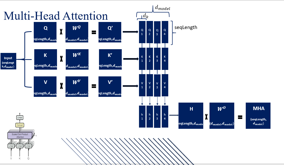
Image source
After performing self-attention for all heads, their outputs are concatenated back together, resulting in a matrix of shape . Finally, this concatenated matrix is projected back to the original embedding dimension using a final learnable matrix , which is of shape . This can be summarized as follows:
After this layer, we apply a skip connection and normalization, just as we did before. The outputs are then fed into the next attention layer, which lies at the heart of the model. As this layer is where the decoder integrates the outputs of the encoder it is therefore called the cross-attention layer.
Cross Attention
Now the cross-attention layer is where the decoder integrates the outputs of the encoder. Instead of performing self-attention solely on the target sequence, the decoder uses the encoder's outputs as the keys and values while the decoder's outputs from the previous layer serve as the queries. The primary goal of the cross-attention layer is to allow the decoder to focus on relevant parts of the input sequence (processed by the encoder) when generating each token of the output sequence.
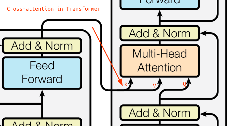
Image source
Therefore, in the cross-attention layer, we use the target embeddings as the queries, which attend to the source sequence embeddings (the keys). The attention mechanism computes the alignment between the source and target sequences. Using the calculated attention weights, we multiply this matrix by the values (i.e., the outputs of the encoder). Again, formulating this mathematically and with the target embeddings and encoder ouput , we get
This operation accumulates information from the encoder, weighted by how much each target token attends to different parts of the source sequence. As usual, after this layer, we add the inputs of the layer to its output as a skip connection. Following this, we apply normalization to the result.
End of the Decoder
Now, before reaching the end of the decoder block, we pass the current values through another feed-forward network (FFN). As with previous layers, we add the input of the FFN to its output via a skip connection and apply normalization to the result. This marks the conclusion of a single decoder block. In practice, we stack multiple decoder blocks in sequence, with each block refining the outputs of the previous one, enabling the model to better capture complex relationships within the data.
Final prediction
Now that we have the outputs of the decoder, we need to map them to probabilities over our vocabulary of tokens. Given the input:
- Source sentence (in English):
src = [976, 6446, 48704, 1072, 290, 8851, 42166, 13] - Target sentence (in German):
trg = [0, 12, 4433, 2304, 8872, 2240, 456, 2349, 13]
We aim to predict the next token for each position in the target sequence. This means our ground truth will be: ground_truth = [12, 4433, 2304, 8872, 2240, 456, 2349, 13, 99999], where 99999 represents the <END> token.
The output of the decoder has a shape of , which contains the contextualized embeddings of each token. However, to generate probabilities over the vocabulary, we need to map these outputs to a new shape: .
This is achieved by applying a linear projection (a dense layer) that transforms the decoder outputs into the vocabulary space. The -th entry of this transformed output will contain the probabilities over all tokens in the vocabulary, representing the likelihood of each token being the next token after token .
Steps:
- Linear Layer: The decoder output is passed through a dense layer with weights of shape to project each token embedding into the vocabulary space.
- Softmax: A softmax operation is applied to the output of the linear layer to compute the probabilities for each token in the vocabulary.
This final output provides a distribution over the vocabulary for each position in the target sequence, enabling the model to predict the next token at each step.
Next up
Now that we understand how a Transformer works internally, in the next post, we will implement one from scratch. There, we will focus on building a translation model, applying the concepts we've explored to transform a source sentence into its corresponding target sentence.