Efficient LLM Finetuning (PEFT) - LoRA and QLoRA explained

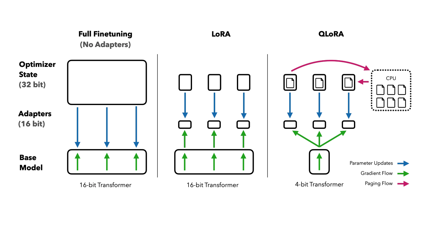
Fine-tuning large language models (LLMs) has emerged as a powerful way to adapt these models to specific tasks or domains, delivering improved performance and tailored behavior. However, this process is not without its challenges. Tradionaly fine-tuning required significant computational resources, often involving extensive GPU hours and large amounts of memory, which can translate into high operational costs. With the advent of (Q)LoRA, fine-tuning large language models has become significantly more cost-effective. In this short blog entry, I will describe the inner workings and underlying theory of (Q)LoRA, explaining how it reduces computational expense while maintaining model performance. All the information compiled here is directly taken from the paper QLoRA: Efficient Finetuning of Quantized LLMs.

Introductory Concepts

To understand the idea behind (Q)LoRA, one must first grasp some fundamental concepts in linear algebra, particularly matrix rank and rank decomposition.

Rank

In linear algebra, the column rank (or row rank) of a matrix $A$ refers to the number of linearly independent columns (or rows) it contains. Mathematically, if $A$ defines a linear map

where $V$ and $W$ are vector spaces, the rank of $A$ is defined as the dimension of the image of $A$:

As already indicated, it can be proven that the column rank and the row rank of a linear map $A$ are in fact equal. Therefore, instead of distinguishing between column or row rank, we simply refer to the quantity $\dim\big(\operatorname{img}(A)\big)$ as rank of $A$.

Rank Decomposition

Now, let $A \in \mathbb{R}^{m \times n}$ be a real-valued matrix with rank $r$. A rank decomposition of $A$ is a factorization of the form

where the matrices $L \in \mathbb{R}^{m \times r}$ and $R \in \mathbb{R}^{r \times n}$ have smaller dimensions. The key insight here is that every finite-dimensional matrix has a rank decomposition.

LoRA (Low-Rank Adaption)

Now we have everything in place to define the process behind LoRA. As we know, each layer of our LLM comprises weights $W \in \mathbb{R}^{d \times d}$ that are tuned to produce a desired output given an input $x \in \mathbb{R}^{d}$. During fine-tuning, our goal is to adjust the weights so that the output better aligns with our preferences. This means that after fine-tuning, we obtain an adjusted weight matrix

such that

The key observation of LoRA is that these weight matrices often contain redundancy and therefore have low rank. If this is the case, we should be able to express

in terms of two smaller matrices

where the rank $r$ satisfies $r \ll d$, such that

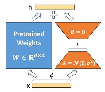
As we can see, this low-rank factorization significantly reduces the number of trainable parameters during fine-tuning, as the pretrained weights remain frozen during fine-tuning (see Figure).

In the figure above, you can see the LoRA adapter — the orange component that gets saved after fine-tuning. The figure also illustrates the initialization scheme used for both low-rank matrices. Instead of initializing both matrices with random noise (which could make the initial steps of training unstable), one matrix is initialized with zeros while the other is initialized with random noise sampled from a Gaussian distribution. This way, their initial product is zero, ensuring that training is not destabilized at the beginning. However, because only one of the matrices is zero, the gradients remain non-zero, allowing the adapter to learn effectively during fine-tuning.

In practice, one often multiplies the LoRA adapter by a scaling factor $\frac{\alpha}{r}$, leading to an update formula of

Although the precise role of $\alpha$ is not fully understood yet, it generally adjusts the overall scale of the low-rank update relative to the original weight $W$. This scaling helps balance the contribution of the adapter during fine-tuning, ensuring that the low-rank modification neither overwhelms nor is negligible compared to the pre-trained weights.

QLoRA (Quantized Low-Rank Adaption)

QLoRA builds upon the concepts of LoRA but incorporates advanced quantization techniques to significantly reduce the memory footprint of fine-tuning. By leveraging low-bit precision representations, QLoRA enables efficient adaptation of large language models while maintaining high performance. To achieve this, QLoRA introduces the following key concepts, with the first two focusing on weight quantization.

NF4 (4-bit NormalFloat) Quantization

The NF4 technique builds upon the idea of quantile quantization, which assigns a quantization bin index to each of a given tensor's weights. Let's, for example, consider the following tensor A of weight values to be quantized using 2-bit quantile quantization:

Using 2-bit quantile quantization, we obtain $2^2 = 4$ distinct bins, meaning:

Given that we have now calculated the centroids of each bin, we can represent the 2-bit quantile quantized tensor $A$ as:

where each index is stored as a 2-bit integer. The calculated centroids, however, are stored in half-precision (float16) or full-precision (float32) in a lookup table.

The problem with this, however, is that the calculation of the quantiles can be very computationally intensive. While there have been proposed algorithms to approximate quantiles, they often incur high quantization errors when encountering outliers.

With NF4, however, we exploit the property of weight distributions, which are often normally distributed with mean $0$ when training neural networks. What we will do now is calculate the $2^k + 1$ quantiles of a normal distribution $N(0, 1)$. We will do this by utilizing the formula

here $Q_X$ refers to the inverse cumulative distribution function (CDF) of the $N(0,1)$ distribution with

where $F_X$ is the CDF of $X$ and $p \in [0,1].$

As you can see, the $q_i$ values are our calculated centroids, which are essentially the averages between consecutive bin boundaries. We will then take the computed $q_i$ and map them into the interval $[-1,1]$. Finally, we take our weight tensor and equally scale it into the interval $[-1,1]$. After that, we can easily quantize the weights to their respective centroids.

One remaining issue is that the initial approach does not guarantee an exact zero centroid. To address this, we allocate quantiles differently for the negative and positive halves of the distribution. Specifically, we use $2^{k-1}$ quantiles for the negative side and $2^{k-1} + 1$ quantiles for the positive side. This ensures that both halves include a quantile corresponding to zero. When we merge these two sets, we remove the duplicate zero quantile so that the final $k$-bit data type contains exactly one zero-valued quantile.

Double Quantization

Before understanding Double Quantization, we must first explore Block-wise k-bit Quantization, which involves compressing data from a high-precision format into a lower-precision one.

To illustrate this, let’s define a full-precision $\texttt{FP32}$ tensor $W^{FP32}$, which we want to quantize into an $\texttt{Int8}$ tensor $W^{Int8}$ with values in the range $[-127,127]$. This transformation is achieved by mapping the full range of $W^{FP32}$ onto $W^{Int8}$ using:

Here, $c\_{\mathrm{FP32}}$ is referred to as the quantization constant. However, this approach has some drawbacks, particularly in the presence of large outlier values.

When a tensor contains extreme outliers, the $\mathrm{absmax}(X\_{\mathrm{FP32}})$ value becomes disproportionately large. This forces the majority of the weights to be mapped to smaller values when scaled, causing most quantized values in $W^{Int8}$ to cluster around zero. As a result, the full 8-bit range is not effectively utilized, leading to reduced precision in weight representation.

To combat this problem, we chunk the tensor into $n$ blocks. We then apply the above quantization process independently to each of the $n$ blocks, resulting in $n$ separate quantization constants.

While this approach introduces additional overhead compared to using a single global constant, it ensures that outliers confined to a single or a few blocks do not negatively impact the 8-bit range utilization of the other blocks. This improves overall precision and prevents most weights from collapsing around zero due to a single extreme value.

Now armed with this knowledge, we can understand the value of the proposed Double Quantization of QLoRA. The goal of Double Quantization is to quantize the quantization constants, which are originally stored in full precision (FP32). QLoRA achieves this by introducing a second constant, $c_2^{\text{FP32}}$, with a block size of 256 to quantize each $c_1^{\text{FP32}}$ to an 8-bit constant, namely $c_1^{\text{FP8}}$.

It is important to note that the block size of 256 for $c_2$ does not correspond to 256 parameters, but rather to 256 quantization constants $c_1$. Each $c_1$ is used for the quantization of 64 parameters, meaning the $c_2$ constants ultimately influence the quantization of $256 \times 64$ parameters.

However, since the $c_1$ constants are all positive, directly applying quantization would not effectively utilize the full 8-bit range. To address this, the mean of each set of $c_1$ constants is subtracted before proceeding with quantization. This centering ensures that the full dynamic range of the 8-bit representation is used efficiently. Now we can see that the single quantization with a block size of 64 will introduce an overhead of

whereas the double quantization will yield an overhead of

Putting everything together

Now that we can put everything we've learned together, we can express the forward pass in a single formula

where

During the forward pass, the quantized weights $W^{\text{NF4}}$ are dynamically dequantized to a working datatype of $\text{BF16}$. Although during LoRA training we only compute gradients with respect to the adapter parameters, $\frac{\partial E}{\partial L_i}$, the computation of these gradients involves the term $\frac{\partial X}{\partial W}$ due to the chain rule. In other words, when we compute

the term $\frac{\partial E}{\partial Y}$ depends on the intermediate activations $X$, which in turn depend on the dequantized weights $W$. Thus, even though only the adapter parameters $L_i$ are updated during training, the overall gradient propagation requires computing $\frac{\partial X}{\partial W}$ in the later layers.

(Q)LoRA Finetuning with Hugginface PEFT

Now that we've covered the theory behind (Q)LoRA-based fine-tuning, let's explore the implementation. Using the Hugging Face PEFT library, we load a model that has been NF4-quantized and fine-tune it with LoRA adapters.

import torch
from transformers import (
    AutoModelForCausalLM,
    AutoTokenizer,
    TrainingArguments,
    Trainer,
    BitsAndBytesConfig,
)
from peft import prepare_model_for_kbit_training, LoraConfig, get_peft_model
from datasets import load_dataset

bnb_config = BitsAndBytesConfig(
    load_in_4bit=True,                  # quantize the model to 4-bit precision
    bnb_4bit_quant_type="nf4",          # use NF4
    bnb_4bit_use_double_quant=True,     # enable double quantization
    bnb_4bit_compute_dtype=torch.bfloat16  # use BF16 for computations
)

model_name = "mistralai/Mistral-7B-v0.1"
tokenizer = AutoTokenizer.from_pretrained(model_name)

model = AutoModelForCausalLM.from_pretrained(
    model_name,
    quantization_config=bnb_config,
    device_map="auto",
)

model = prepare_model_for_kbit_training(model)
lora_config = LoraConfig(
    r=16,
    lora_alpha=8,
    target_modules=["all-linear"],
    lora_dropout=0.05,
    bias="none",
    task_type="CAUSAL_LM"
)

model = get_peft_model(model, lora_config)

dataset = load_dataset("wikitext", "wikitext-2-raw-v1")

def tokenize_function(examples):
    return tokenizer(examples["text"], truncation=True, max_length=512)

tokenized_dataset = dataset.map(tokenize_function, batched=True, remove_columns=["text"])

training_args = TrainingArguments(
    output_dir="./qlora_finetuned_model",
    per_device_train_batch_size=4,
    per_device_eval_batch_size=4,
    num_train_epochs=3,
    learning_rate=2e-4,
    logging_steps=10,
    save_steps=100,
    evaluation_strategy="steps",
    fp16=True,  # mixed precision training
    report_to="none",
)

trainer = Trainer(
    model=model,
    args=training_args,
    train_dataset=tokenized_dataset["train"],
    eval_dataset=tokenized_dataset["validation"],
)

trainer.train()

model.save_pretrained("./qlora_finetuned_model_final")

As you can see, we aim to fine-tune the "mistralai/Mistral-7B-v0.1" model on the wikitext-2-raw-v1 dataset. Eventough this dataset was likely part of the model's original training, we just don't care.

To achieve QLoRA based fine-tuning, we use bitsandbytes to quantize the model to 4-bit precision.

bnb_config = BitsAndBytesConfig(
    load_in_4bit=True,                  # Quantize the model to 4-bit precision
    bnb_4bit_quant_type="nf4",          # Use NF4 quantization
    bnb_4bit_use_double_quant=True,     # Enable double quantization
    bnb_4bit_compute_dtype=torch.bfloat16  # Use BF16 for computations
)

These parameters cover everything needed for QLoRA fine-tuning, as discussed earlier.

Next, we prepare the LoRA configuration:

lora_config = LoraConfig(
    r=16,
    lora_alpha=8,
    target_modules=["all-linear"],
    lora_dropout=0.05,
    bias="none",
    task_type="CAUSAL_LM"
)

Here, we set the rank of the adapters to 16 and the value of $\alpha$ to 8. The target_modules variable determines which layers will be fine-tuned using LoRA. In this case, we apply LoRA to all linear layers, but we could also specify individual layers, such as attention layers. The following lines are straightforward. They handle dataset preparation through tokenization and set up the Trainer class with reasonable parameters. These configurations should already be familiar from my previous posts 🤓