- Published on
Introduction to Transformers - Part 02 - Llama 3 - Building a LLM from scratch
- Authors

- Name
- Jan Hardtke
Meta has recently announced the release of LLaMA 3.3, the latest iteration in their state-of-the-art open-source foundational large language models (LLMs).

This new version, particularly the LLaMA 3.3 70B model, demonstrates remarkable performance that either matches or surpasses the capabilities of OpenAI's closed-source GPT-4o across a wide range of benchmarks. LLaMA 3 represents a significant leap in large language model development, building upon Meta's ongoing commitment to open-source AI innovation. In this blog post, we will look at the architectural advancements and optimizations that set LLaMA 3 apart from earlier models and the original transformer framework.
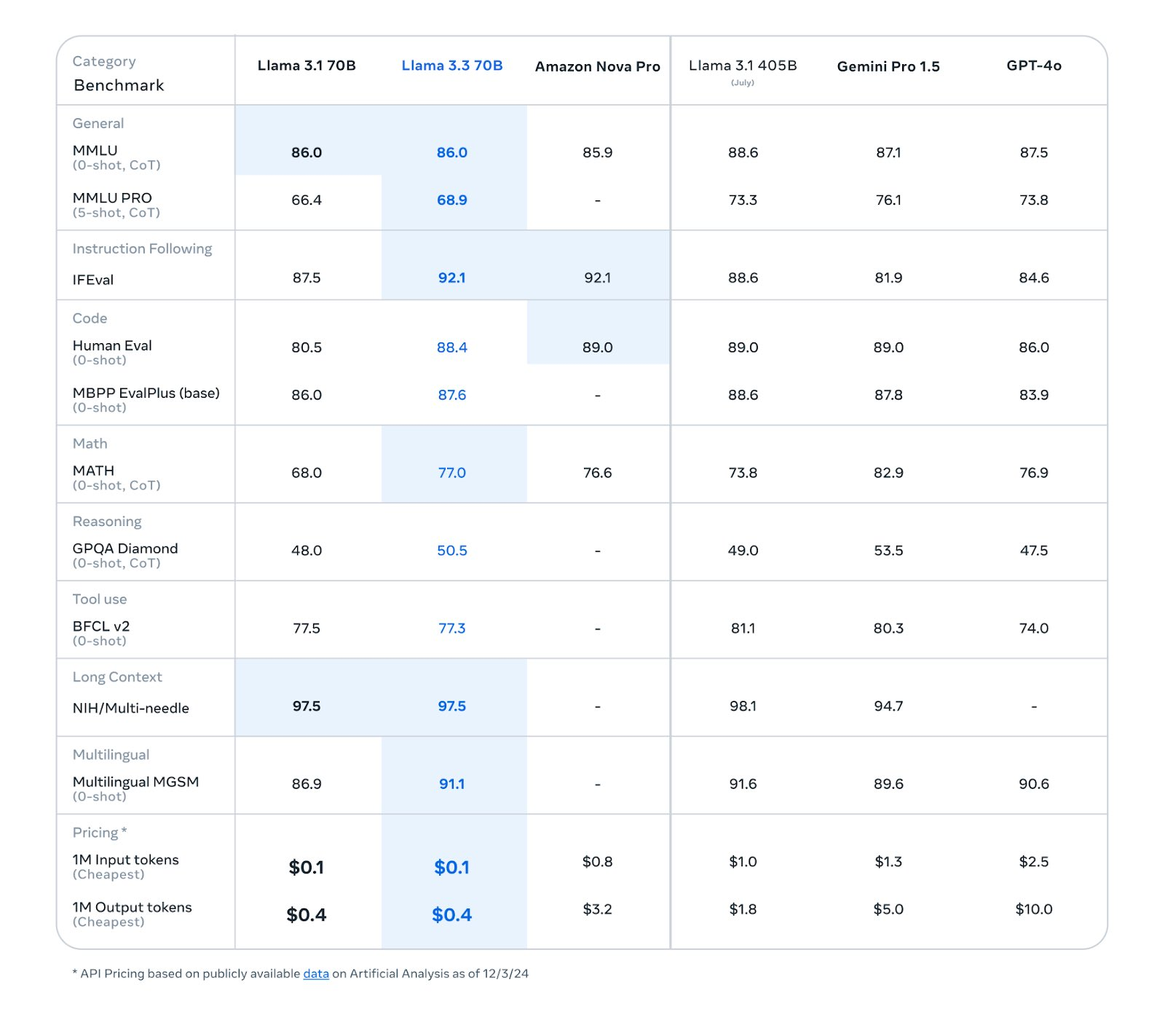
Image source
Prerequisites
Before diving into the model's code, we will first explore the most significant architectural innovation introduced in Llama 3.
Rotary positional Encodings (RoPE)
Rotary Position Embeddings (RoPE) are an advanced method for encoding positional information in transformer models, designed to enhance their ability to process sequential data. Unlike fixed or learned positional embeddings, RoPE introduces a rotational transformation in the query and key vectors of the self-attention mechanism. This approach embeds positional relationships directly into the angular components of these vectors, allowing the model to generalize better across different sequence lengths and maintain relative positional information.
Given the vectors and , which represent the embedded vectors of a word at positions and in a sequence, the self-attention mechanism between these tokens at different positions is defined by or , depending on whether the configuration is row-wise or column-wise.
To incorporate relative positional information, we aim to express the inner product of the query vector and the key vector as a function . This function should depend solely on the word embeddings and , as well as their relative position . In other words, the inner product should encode positional information solely in a relative manner:
The primary objective is to devise an encoding mechanism such that the functions and align with and satisfy this relationship.
This is illustrated in the exemplary figure below. The later the word "dog" appears in the sentence, the more it is rotated. However, the most important observation is that the rotation angle between two word vectors (e.g., between "pig" and "dog") remains consistent if their relative distance stays the same, regardless of their absolute position or the length of the sentence. This is what the existence of such a function implies.

Image source
To derive RoPE, we will focus on the case where and are 2-dimensional. We define their positionally encoded counterparts as:
where and denote their positions, such that:
Additionally, we define the initial conditions for as:
To find solutions for and , we note that our vectors and are 2-dimensional. This allows us to represent them as a complex number using Euler's formula:
Using this representation, we can define , , and as follows:
Here, represents the magnitude (scaling factor) and represents the phase (angle of rotation) for the respective functions. This complex representation elegantly encodes both magnitude and phase, enabling us to incorporate relative positional information. As we want to satisfy , we can derive the following eqautions for the radial and phase functions and :
The derivation of the first one is indeed trival. The equality can be derived as follows:
In this representation, our initial conditions can be defined as:
With the following relationships:
and
Now, setting and leveraging our knowledge about the initial conditions, we obtain:
From this, we can observe that a possible straight forward solution for , , and can be derived as follows:
From this, we can see that these solutions for , , and are, in fact, independent of any positional information.
Additionally, we observe that in is independent of or . Since , there must exist some function such that:
Now let’s set , which means we get
As is constant, we can write as
with and .
This means when now have a way to write our encoding functions and :
As we dont make assumtions about and we choose
Therefore we can derive the following solution:
Instead of using Euler's formula with complex numbers, we can express rotations in the attention mechanism using rotation matrices. Let's define a rotation matrix which rotates 2D vectors by :
We can now rewrite and as follows:
Using this matrix representation, the standard attention mechanism can be expressed as:
the last equality highlights a crucial point: the applied rotation depends solely on the distance between tokens () and not on the sentence length or absolute token positions
Currently, we have only considered 2D vectors for and . To generalize this to , we divide the -dimensional vector into two-dimensional subspaces. Each subspace is rotated based on the position of the token in the sequence.
Now given a , we formulate a , with:
with pre-defined parameters:
This approach takes every pair of and independently rotates it based on the position and the index of the pair in ().
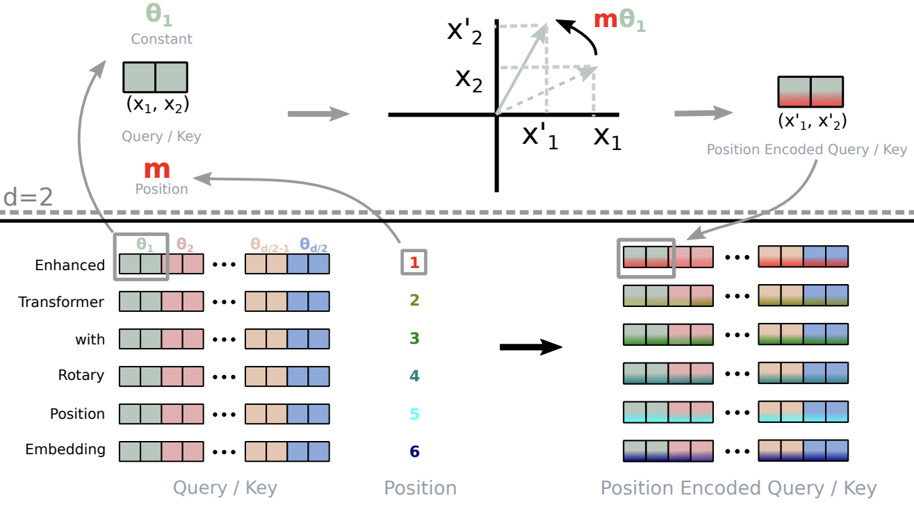
Image source
The above figure illustrates this process. For each token embedding, we take successive 2D subvectors and rotate them by a predefined angle , where is the index of the subvector within the token embedding, multiplied by , the position of the token in the sequence.
Note that the above formulation of is highly inefficient, as it constructs a mostly empty matrix. Therefore, the paper introduces very simple elementwise vector operations, which are equivalent to multiplying with the very sparse . It defines
Now this is the operation that we will implement later in PyTorch.
Grouped-Query Attention (GQA)
Grouped Query Attention (GQA) is an optimization technique in attention mechanisms, aimed at reducing the computational complexity of standard multi-head attention. Instead of computing a separate query for each head, GQA groups multiple heads together to share a single query representation.
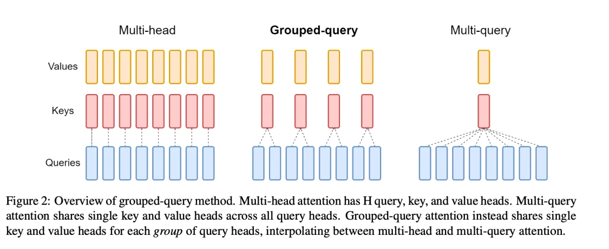
Image source
The above figure illustrates this clearly. Each rectangle in the figure represents one attention head. In standard attention, each head in the queries attends to the corresponding head in the keys. However, in this approach, multiple query heads are grouped together to attend to a single key head. The standart attention mechanism can be expressed as:
where:
- is the input sequence of token embeddings,
- are the weight matrices for the query, key, and value, respectively,
- are the computed query, key, and value matrices,
- is the sequence length, and is the embedding dimension.
Here, , where is the head dimension. In practice, , as we later reshape the , , and tensors into the shape:
The fundamental difference in GQA lies in the shape of the weight matrices. In standard attention, the weight matrices are of size:
where .
In GQA, the weight matrices for and are of size:
where refers to the number of key-value heads. For a group size of , as shown in the figure, the number of key-value heads is reduced:
This will result in the shape for our . Such that we can reshape them into:
Now, since , we observe that by sharing attention heads between queries, we can drastically reduce the memory footprint.
Preparing the Dataset
We will train out Llama model on the TinyStories datasets. The TinyStories dataset is a dataset of short, narrative-style stories designed to be used for training natural language processing (NLP) models, particularly language models like Llama. These dataset consist of small, self-contained stories that capture a variety of writing styles, including simple plots, dialogues, and events, making them suitable for fine-tuning language models on tasks related to story generation. This is a small example from the TinyStories dataset:
Once upon a time, there was a little car named Beep. Beep loved to go fast and play in the sun. Beep was a healthy car because he always had good fuel. Good fuel made Beep happy and strong. One day, Beep was driving in the park when he saw a big tree. The tree had many leaves that were falling. Beep liked how the leaves fall and wanted to play with them. Beep drove under the tree and watched the leaves fall on him. He laughed and beeped his horn. Beep played with the falling leaves all day. When it was time to go home, Beep knew he needed more fuel. He went to the fuel place and got more healthy fuel. Now, Beep was ready to go fast and play again the next day. And Beep lived happily ever after.
Now let’s look our code that prepares this dataset for training:
import torch
from datasets import load_dataset

torch.set_printoptions(profile="full")
from datasets import load_dataset
from transformers import GPT2TokenizerFast
from model import Llama3, ModelArgs
from transformers import DataCollatorForLanguageModeling
from torch.utils.data import DataLoader
import logging

logging.basicConfig(
    level=logging.INFO,
    format="%(asctime)s %(levelname)s: %(message)s",
    handlers=[logging.StreamHandler()],  # Logs to stdout
)
logger = logging.getLogger()

device = torch.device("cuda" if torch.cuda.is_available() else "cpu")

max_seq_len = 256
batch_size = 70
dataset = load_dataset("roneneldan/TinyStories", split="train").select(range(1000))
tokenizer = GPT2TokenizerFast.from_pretrained("gpt2")
tokenizer.add_special_tokens({"pad_token": "[PAD]"})


def tokenize_function(examples):
    return tokenizer(examples["text"], max_length=max_seq_len, truncation=True)


dataset = dataset.filter(
    lambda example: example["text"] is not None and example["text"].strip() != ""
)

tokenized_dataset = dataset.map(
    tokenize_function, batched=True, remove_columns=["text"]
)

data_collator = DataCollatorForLanguageModeling(tokenizer=tokenizer, mlm=False)

dataloader = DataLoader(
    tokenized_dataset,
    batch_size=batch_size,
    shuffle=True,
    collate_fn=lambda feature: Llama3.gen_labels(feature, tokenizer, data_collator),
)
This loads the TinyStories dataset and prepares it for training a language model. It tokenizes the text using GPT2TokenizerFast, ensuring that the sequences are of a fixed length (max_seq_len). The dataset is filtered to remove empty or invalid texts. A DataLoader is created using a custom collate function (Llama3.gen_labels) to generate labels for training, while efficiently handling batch processing with DataCollatorForLanguageModeling, which pads sequences and generates attention masks.
class Llama3
  (...)
  @staticmethod
  def __build_masks(seq_len, attention_mask, device, position=0, training=False):
      causal = torch.tril(torch.ones(seq_len, seq_len, dtype=torch.bool)).unsqueeze(0)
      (...)
      if attention_mask == None:
          return causal
      attention_mask = attention_mask.unsqueeze(1).repeat(1, seq_len, 1).int()

      return (causal & attention_mask).int()

  @staticmethod
  def gen_labels(labels, tokenizer, data_collator, ignore_index=-100):
      batch = data_collator(labels)
      labels = batch["labels"]
      attention_mask = batch["attention_mask"]
      for i in range(labels.shape[0]):
          l = torch.roll(labels[i], -1)
          target_indices = (l == ignore_index).nonzero(as_tuple=True)[0]
          if len(target_indices) == 0:
              l[-1] = tokenizer.eos_token_id
          else:
              seq_len = len(l) - len(target_indices)
              l[-1] = ignore_index
              l[seq_len - 1] = tokenizer.eos_token_id

          labels[i] = l

      batch["labels"] = labels
      batch["attention_mask"] = Llama3.__build_masks(
          labels.shape[1], attention_mask, device, training=True
      )
  (...)
The gen_labels function is designed to prepare the labels for training by shifting them one token to the left and appending an EOS (End of Sequence) token at the end. At the start of the function, the labels are just a copy of the input. The challenge is to place the EOS token at the correct position, which requires determining the length of the unpadded sequence. If padding is present, the function places the EOS token at the end of the actual data, not on top of padding tokens. If no padding exists, the EOS token is placed at the very end of the sequence.
Once the labels are shifted and the EOS token is placed correctly, the function must handle the attention masks. Since DataCollatorForLanguageModeling provides an array of attention values for a single sequence, the function needs to convert this into a matrix that can be used for causal language modeling. This involves combining the attention mask with a causal mask, which is a lower triangular matrix, ensuring that the model only attends to previous tokens in the sequence and not to any future tokens.
Llama3 - Model Architecture
Llama3 Architecture Overview
Now that we have everything in place, let's look at how the Llama3 architecture is structured. Below is an overview of its design:
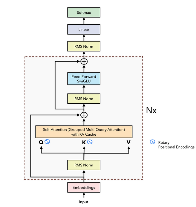
Image source
As we can see, Llama3 is conceptually very similar to the vanilla transformer architecture. Most importantly, the Llama3 and other GPT-style models only consist of a decoder-only transformer. This means that we won't use the encoder and the cross-attention, which we covered in the previous blog post. Another notable change that stands out is the use of RMSNorm instead of LayerNorm for normalization.
While LayerNorm normalizes the input by using the mean and standard deviation of the tensor, RMSNorm uses the root mean square of the elements, making it simpler and computationally more efficient. Both methods have learnable scaling and bias parameters, but RMSNorm avoids the need for computing the mean and standard deviation, which can be more efficient in practice.
Additionally, we observe that the positional encoding (RoPE) is applied directly to the queries and keys in the attention layer, rather than at the embedding level. The values, however, are not position encoded.
After that the outputs of the attention layer are again feed into a FFN. This time however we use the so called SwiGLU activation function. The SwiGLU (Swish-Gated Linear Unit) activation function is a variation of the standard activation functions like ReLU and GELU. It is designed to combine the benefits of the Swish activation function and the Gated Linear Unit (GLU). SwiGLU introduces a gating mechanism using a linear function combined with the Swish activation, which helps improve model performance, particularly in transformer-based architectures.
The SwiGLU activation function is mathematically defined as:
Where:
is the Swish activation function defined as:
with being the sigmoid function:
is the Gated Linear Unit with: with being the element-wise product
Now that we have an overview of the Llama3 architecture, let's quickly discuss the implementation of the rotary positional encodings in our model. As mentioned earlier, the direct formulation of a large, mostly empty matrix for positional encodings is inefficient and wasteful in terms of memory and computation. Therefore, we pursue a different approach to implement positional encodings.
Below we have the RoPE-class, which implents the positional encoding.
class RoPE:
    @staticmethod
    def compute_freq(head_dim: int, seq_len: int, base: int = 10000):
        exp = -2 * torch.arange(0, head_dim, 2).float() / head_dim
        thetas = torch.pow(base, exp)
        m = torch.arange(0, seq_len).float()
        freq = torch.outer(m, thetas).float()
        freq_comp = torch.polar(torch.ones_like(freq), freq)
        return freq_comp

    @staticmethod
    def apply_rotary_embedding(x: torch.Tensor, freq_cis):
        # batch,seq_len,heads,d_k
        x_comp = torch.view_as_complex(x.float().reshape(*(x.shape[:-1]), -1, 2))
        freq_com = freq_cis.unsqueeze(0).unsqueeze(2)

        x_out = torch.view_as_real(x_comp * freq_com).reshape(*x.shape)
        return x_out.float()
The compute_freq function precomputes the for and .
While the first two lines implement the following equation:
the third line implements the outer product between the array of positions and the .
Lastly, we use torch.polar, which converts the number into a complex number using the matrix entries as angular components. Mathematically, this whole process can be expressed as:
After the torch.polar operation, which converts the matrix entries into their polar representation, it looks like this:
As we can see the radial components are .
We will now shift our focus on the apply_rotary_embedding function, which given queries and keys , will encode them based on their position in the sentence.
let’s demonstrate this problems bei focusing on , which contains the angular components for position . Let be the queries () and keys(). We will transfrom them in the following way:
Now we take this vector of complex entries and multiply it element-wise with :
We can now view this result again as a real matrix and reshape it into its original dimension:
As we can see, we arrived at our end result of , with the operations performed in our PyTorch code in the function apply_rotation.
Now that we have covered the most important details that distinguish the Llama3 architecture from a vanilla decoder-only transformer, we can actually take a look at the code of the Llama class.
class FFN(nn.Module):
    def __init__(self, d_model=256, multiple_of=256):
        super(FFN, self).__init__()
        hidden = 4 * d_model
        hidden = int(2 * hidden / 3)

        hidden = multiple_of * ((hidden + multiple_of - 1) // multiple_of)
        self.w1 = nn.Linear(d_model, hidden, bias=False)
        self.v = nn.Linear(d_model, hidden, bias=False)
        self.w2 = nn.Linear(hidden, d_model, bias=False)

    def forward(self, x):
        return self.w2(nn.functional.silu(self.w1(x)) * self.v(x))

class MultiHeadGQAttention(nn.Module):
    flash = False

    def __init__(self, heads=4, d_model=256, group_size=2, max_seq_len=256):
        super(MultiHeadGQAttention, self).__init__()
        self.heads = heads
        self.d_model = d_model
        self.group_size = group_size

        self.W_q = nn.Linear(d_model, d_model, bias=False)
        self.W_k = nn.Linear(d_model, d_model // group_size, bias=False)
        self.W_v = nn.Linear(d_model, d_model // group_size, bias=False)
        self.W_o = nn.Linear(d_model, d_model, bias=False)

    def forward(
        self,
        q,
        k,
        v,
        mask,
        freq_cis,
        position=-1,
    ):
        d_k = self.d_model // self.heads
        bs, seq_len = q.shape[:2]
        q, k, v = self.W_q(q), self.W_k(k), self.W_v(v)

        q = q.view(
            q.shape[0], q.shape[1], self.heads, -1
        )  # (batch,seq_len,heads,d_k) or (batch,1,heads,d_k)
        k = k.view(
            k.shape[0], k.shape[1], self.heads // self.group_size, -1
        )  # (batch,seq_len,heads,d_k) or (batch,1,heads,d_k)
        v = v.view(
            v.shape[0], v.shape[1], self.heads // self.group_size, -1
        )  # (batch,seq_len,heads,d_k) or (batch,1,heads,d_k)
        q = RoPE.apply_rotary_embedding(q, freq_cis)
        k = RoPE.apply_rotary_embedding(k, freq_cis)
        if not self.training:
            k, v = self.kv_cache.update(k, v, position)


        q, k, v = (x.transpose(1, 2) for x in (q, k, v))

        if MultiHeadGQAttention.flash:
            q, k, v = (x.contiguous() for x in (q, k, v))
            output = (
                F.scaled_dot_product_attention(
                    q, k, v, attn_mask=(mask == 1).unsqueeze(1)
                )
                .transpose(1, 2)
                .reshape(bs, seq_len, -1)
            )
        else:
            scores = torch.matmul(q, k.transpose(-2, -1)) / math.sqrt(d_k)
            if mask is not None:
                mask = mask.unsqueeze(1)
                scores = torch.masked_fill(scores, mask == 0, float("-inf"))
                attention = nn.functional.softmax(scores, dim=-1)
                output = (
                    torch.matmul(attention, v)
                    .transpose(1, 2)
                    .contiguous()
                    .view(bs, seq_len, -1)
                )

        output = self.W_o(output)
        return output

class DecoderLayer(nn.Module):
    def __init__(self, d_model=256, heads=4, group_size=2, max_seq_len=256):
        super(DecoderLayer, self).__init__()
        self.norm1 = nn.RMSNorm(d_model, eps=1e-6)
        self.norm2 = nn.RMSNorm(d_model, eps=1e-6)
        self.ffn = FFN(d_model=d_model)
        self.attention = MultiHeadGQAttention(
            heads=heads, d_model=d_model, group_size=group_size, max_seq_len=max_seq_len
        )

    def forward(self, x, tgt_causal_mask, pos, freqs_cis):
        x_norm = self.norm1(x)
        x = x + self.attention(
            x_norm, x_norm, x_norm, tgt_causal_mask, freqs_cis, position=pos
        )
        return x + self.ffn(self.norm2(x))

class Llama3(nn.Module):
    def __init__(self, params: ModelArgs):
        super(Llama3, self).__init__()
        self.tokenizer = params.tokenizer
        self.max_seq_len = params.max_seq_len
        self.ignore_index = params.ignore_index
        self.num_layers = params.num_layers
        self.layers = nn.ModuleList(
            [
                DecoderLayer(
                    d_model=params.d_model,
                    heads=params.heads,
                    group_size=params.group_size,
                    max_seq_len=params.max_seq_len,
                )
                for _ in range(params.num_layers)
            ]
        )
        self.embedding = nn.Embedding(params.vocab_size, params.d_model)
        self.norm = nn.RMSNorm(params.d_model, eps=1e-6)
        self.ffn = nn.Linear(params.d_model, params.vocab_size, bias=False)

        self.d_k = params.d_model // params.heads
        self.freqs_cis = RoPE.compute_freq(
            head_dim=params.d_model // params.heads, seq_len=params.max_seq_len
        )
        self.d_model = params.d_model

        MultiHeadGQAttention.flash = params.use_flash
    (...)
    def calc_loss(self, logits, labels):
        loss = nn.functional.cross_entropy(
            logits.view(-1, logits.shape[-1]),
            labels.view(-1),
            ignore_index=self.ignore_index,
        )
        return loss

    def __run_model(self, tgt, attention_mask, position=0):

        tgt_embed = self.embedding(tgt)
        freqs_cis = self.freqs_cis[position : position + tgt_embed.shape[1]].to(
            tgt.device
        )

        for i in range(self.num_layers):
            tgt_embed = self.layers[i](tgt_embed, attention_mask, position, freqs_cis)
        return self.ffn(self.norm(tgt_embed))

    def forward(self, tgt, attention_mask, labels):
        logits = self.__run_model(tgt, attention_mask)
        return self.calc_loss(logits, labels)
As this is rather much to comprehend, we will start with the forward method of the Llama class. It is easy to see that this just calls __run_model, which precomputes the frequency components for the position encoding, based on the position of the current token. This is a result of the KV-Cache, which we will cover in a bit. The determined are then passed to the decoder layers, together with the token embeddings and masks.
The DecoderLayer may be of more interest:
class DecoderLayer(nn.Module):
    def __init__(self, d_model=256, heads=4, group_size=2, max_seq_len=256):
        super(DecoderLayer, self).__init__()
        self.norm1 = nn.RMSNorm(d_model, eps=1e-6)
        self.norm2 = nn.RMSNorm(d_model, eps=1e-6)
        self.ffn = FFN(d_model=d_model)
        self.attention = MultiHeadGQAttention(
            heads=heads, d_model=d_model, group_size=group_size, max_seq_len=max_seq_len
        )

    def forward(self, x, tgt_causal_mask, pos, freqs_cis):
        x_norm = self.norm1(x)
        x = x + self.attention(
            x_norm, x_norm, x_norm, tgt_causal_mask, freqs_cis, position=pos
        )
        return x + self.ffn(self.norm2(x))
As we can see from our architecture overview from before, we first do an RMSNorm before we feed the output into the MultiHeadGQAttention layer. Applying the skip connection and the FFN is pretty self explanotroy. So the most interesting Layer is the MultiHeadGQAttention. So let’s look at that:
class MultiHeadGQAttention(nn.Module):
    flash = False

    def __init__(self, heads=4, d_model=256, group_size=2, max_seq_len=256):
        super(MultiHeadGQAttention, self).__init__()
        self.heads = heads
        self.d_model = d_model
        self.group_size = group_size

        self.W_q = nn.Linear(d_model, d_model, bias=False)
        self.W_k = nn.Linear(d_model, d_model // group_size, bias=False)
        self.W_v = nn.Linear(d_model, d_model // group_size, bias=False)
        self.W_o = nn.Linear(d_model, d_model, bias=False)

    def forward(
        self,
        q,
        k,
        v,
        mask,
        freq_cis,
        position=-1,
    ):
        d_k = self.d_model // self.heads
        bs, seq_len = q.shape[:2]
        q, k, v = self.W_q(q), self.W_k(k), self.W_v(v)

        q = q.view(
            q.shape[0], q.shape[1], self.heads, -1
        )  # (batch,seq_len,heads,d_k) or (batch,1,heads,d_k)
        k = k.view(
            k.shape[0], k.shape[1], self.heads // self.group_size, -1
        )  # (batch,seq_len,heads,d_k) or (batch,1,heads,d_k)
        v = v.view(
            v.shape[0], v.shape[1], self.heads // self.group_size, -1
        )  # (batch,seq_len,heads,d_k) or (batch,1,heads,d_k)
        q = RoPE.apply_rotary_embedding(q, freq_cis)
        k = RoPE.apply_rotary_embedding(k, freq_cis)
        if not self.training:
            k, v = self.kv_cache.update(k, v, position)


        q, k, v = (x.transpose(1, 2) for x in (q, k, v))

        if MultiHeadGQAttention.flash:
            q, k, v = (x.contiguous() for x in (q, k, v))
            output = (
                F.scaled_dot_product_attention(
                    q, k, v, attn_mask=(mask == 1).unsqueeze(1)
                )
                .transpose(1, 2)
                .reshape(bs, seq_len, -1)
            )
        else:
            scores = torch.matmul(q, k.transpose(-2, -1)) / math.sqrt(d_k)
            if mask is not None:
                mask = mask.unsqueeze(1)
                scores = torch.masked_fill(scores, mask == 0, float("-inf"))
                attention = nn.functional.softmax(scores, dim=-1)
                output = (
                    torch.matmul(attention, v)
                    .transpose(1, 2)
                    .contiguous()
                    .view(bs, seq_len, -1)
                )

        output = self.W_o(output)
        return output
As we can see, this is standard functionality, with most parts being identical to the standard attention layer used in a decoder-only Transformer. However, the first difference arises in the weight matrices for , , and . Specifically, we choose and to have dimensions , where .
In the method, we use a standard reshaping mechanism to ensure that the resulting tensors for , , and have the shape .
Next, we apply positional encoding to the queries and keys using the previously defined function. As mentioned earlier, the contain the terms , where represents the positions of the tokens fed into the model. This step is crucial, especially during inference, as the entire sequence of tokens is not fed into the model repeatedly. We will delve into this aspect in more detail later.
Following this, we perform the now well-known attention operation between the encoded , , and the plain . Additionally, there is an optional function called . This function provides a hardware- and memory-efficient implementation of the attention operation, commonly referred to as flash attention.
We will not go into much detail about flash attention in this post, but we may cover it in another post. For now, it suffices to say that this function implements attention more efficiently in terms of both hardware and memory usage.
Now this already completes the model code of Llama! We will use the following training code, along with the data preparation code from above, to make our tiny model tell us some stories!
warmup = 100
lr = 1e-4
min_lr = 7e-5

args = ModelArgs(
    vocab_size=len(tokenizer),
    tokenizer=tokenizer,
    d_model=256,
    heads=16,
    group_size=2,
    num_layers=32,
    max_seq_len=max_seq_len,
    use_flash=True,
)


epochs = 2

model = Llama3(args).to(device)
# model.load_state_dict(torch.load('tiny_stories_2.pth'))
model = torch.compile(model)
model.train()
optim = torch.optim.AdamW(model.parameters(), lr=lr, betas=(0.9, 0.999), weight_decay=0)
# lr_scheduler = InverseSquareRootLR(optim, warmup, lr, min_lr=min_lr)
logger.info(
    f"Param. count: {sum(p.numel() for p in model.parameters() if p.requires_grad)}"
)
scaler = torch.GradScaler()

for epoch in range(epochs):
    for i, batch in enumerate(dataloader):

        inputs = batch["input_ids"].to(device)
        labels = batch["labels"].to(device)
        attention_mask = batch["attention_mask"].to(device)

        optim.zero_grad()

        with torch.autocast(device_type="cuda", dtype=torch.bfloat16):
            loss = model(inputs, attention_mask, labels)

        scaler.scale(loss).backward()

        scaler.unscale_(optim)
        torch.nn.utils.clip_grad_norm_(model.parameters(), max_norm=1.0)

        scaler.step(optim)
        scaler.update()
        # lr_scheduler.step()

        logger.info(
            f"Epoch [{epoch+1}/{epochs}], Step [{i+1}/{len(dataloader)}], Loss: {loss.item():.4f}"
        )
        if (i + 1) % 1000 == 0:
            torch.save(model._orig_mod.state_dict(), "tiny_stories_50M.pth")
As you can see, there is nothing special about this code. We set up our optimizer, compile our Llama3 model, and feed the inputs and labels, such as the attention mask, into the model. Additionally, we use the package, which provides methods for implementing mixed-precision training.
Now that we have set up our training code, trained, and subsequently saved our model to , we can actually use this model to sample some stories from it. So let's do that!
Optimizing Inference - The KV-Cache
One of the most important optimizations that Llama has introduced in their architecture is the so-called key-value cache. The purpose of this becomes clear if we look at the figure below:
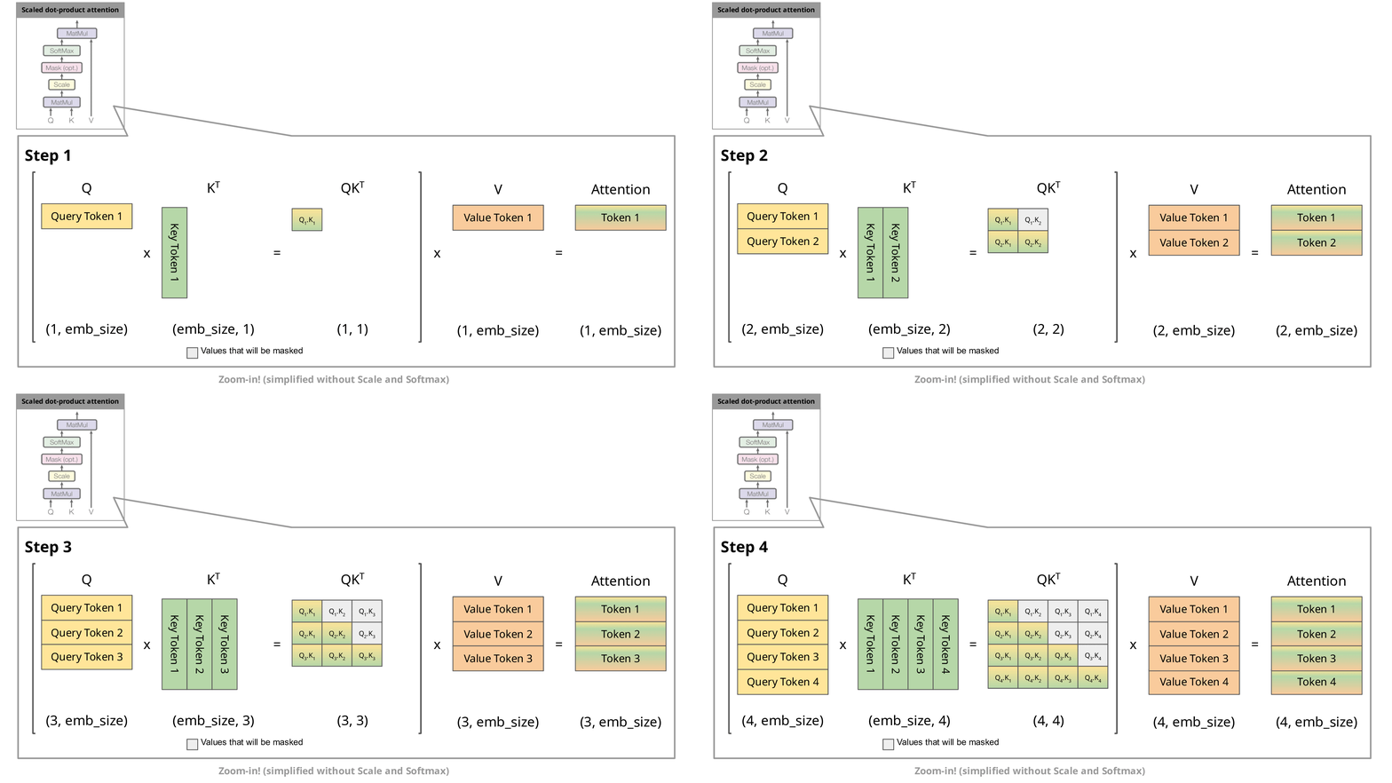
Image source
As you know, during inference we sample the next token and append it to the sequence before we feed this new sequence into the transformer to predict the next token. But as you can see in the figure, to predict token 5, we only need query token 4 to multiply with the keys. This means to predict token 5, we only need the last row of the attention matrix. Thus, instead of feeding in the entire sequence of tokens of length to predict , we just feed in the -th token. For the attention and subsequent multiplication with , however, we still need the previous tokens. This is exactly where the key-value cache (kv-cache) comes in.
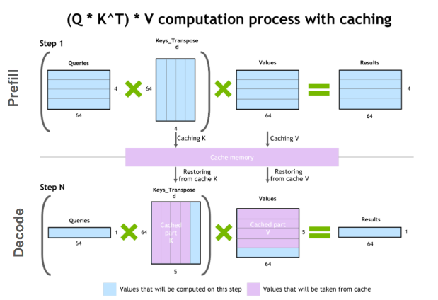
Image source
For every token we see, we save it in the kv-cache for later usage in the multiplications. By doing this, we can save a significant amount of attention multiplications, as we only need to compute the last row of the attention matrix! Nice!
Now lets look at the code for the KV-Cache:
class KV_Cache(nn.Module):
    def __init__(self, batch_size, seq_length, n_kv_heads, head_dim):
        super(KV_Cache, self).__init__()
        device = "cuda"
        cache_shape = (batch_size, seq_length, n_kv_heads, head_dim)
        self.cache_k = torch.zeros(cache_shape, device=device)
        self.cache_v = torch.zeros(cache_shape, device=device)

    def update(self, xk, xv, pos):
        bx, seq_len = xk.shape[:2]
        self.cache_k[:bx, pos : pos + seq_len] = xk
        self.cache_v[:bx, pos : pos + seq_len] = xv
        return self.cache_k[:bx, : pos + seq_len], self.cache_v[:bx, : pos + seq_len]
Here we reserve as much space as we could possibly need by constructing a zero tensor of shape (batch_size, max_seq_length, n_kv_heads, head_dim). Then, during the update, we pass in the current token position and save the keys and values into the cache before returning all the cached values up to the current point in time.
Here is how we will use it in the class:
class MultiHeadGQAttention(nn.Module):
    flash = False
    def __init__(self, heads=4, d_model=256, group_size=2, max_seq_len=256):
        super(MultiHeadGQAttention, self).__init__()
        (...)
        self.kv_cache = KV_Cache(
            batch_size=4,
            seq_length=max_seq_len,
            n_kv_heads=self.heads // self.group_size,
            head_dim=d_model // heads,
        )

    def __repeat_kv(self, x):
        bs, slen, n_kv_heads, head_dim = x.shape
        return (
            x[:, :, :, None, :]
            .expand(bs, slen, n_kv_heads, self.group_size, head_dim)
            .reshape(bs, slen, n_kv_heads * self.group_size, head_dim)
        )
    def forward(
        self,
        q,
        k,
        v,
        mask,
        freq_cis,
        position=-1,
    ):
        (...)
        q = RoPE.apply_rotary_embedding(q, freq_cis)
        k = RoPE.apply_rotary_embedding(k, freq_cis)
        if not self.training:
            k, v = self.kv_cache.update(k, v, position)

        k = self.__repeat_kv(k)
        v = self.__repeat_kv(v)
        (...)
As you can see, we will store the keys and values in the cache after we positional encoded them. Now lets look at the function, that actually handles sampling from the model, utilizing the kv-cache:
 def generate_kv(self, prompt, tokenizer, temp=1.0, top_p=None):
        device = "cuda"
        tokenized = tokenizer(prompt, max_length=self.max_seq_len, truncation=True)
        tokens = torch.tensor(tokenized["input_ids"]).unsqueeze(0).to(device)
        sampled_token = None
        sampled_tokens = tokens.squeeze(0).tolist()

        token_len = tokens.shape[1]

        mask = (
            torch.tril(torch.ones(token_len, token_len, dtype=torch.bool))
            .unsqueeze(0)
            .to(device)
        )
        i = 0
        for block in self.layers:
            block.attention.cache = KV_Cache(
                batch_size=1,
                seq_length=self.max_seq_len,
                n_kv_heads=self.heads // self.group_size,
                head_dim=self.d_model // self.heads,
            )
        while i < self.max_seq_len:

            logits = self.__run_model(tokens, mask, position=i)[:, -1, :] / temp
            probabilities = F.softmax(logits.float(), dim=-1).squeeze()
            if top_p is not None:
                sorted_probs, sorted_indices = torch.sort(
                    probabilities, descending=True
                )
                cumulative_probs = torch.cumsum(sorted_probs, dim=-1)
                cutoff_index = torch.searchsorted(cumulative_probs, top_p, right=True)

                sorted_probs[cutoff_index + 1 :] = 0
                sorted_probs = sorted_probs / sorted_probs.sum()
                probabilities = torch.zeros_like(probabilities).scatter(
                    0, sorted_indices, sorted_probs
                )

                sampled_token = torch.multinomial(probabilities, num_samples=1)
            else:
                sampled_token = torch.multinomial(probabilities, num_samples=1)

            tokens = sampled_token.unsqueeze(0)
            if sampled_token.item() != tokenizer.eos_token_id:
                sampled_tokens.append(sampled_token.item())
            else:
                break
            i = len(sampled_tokens)
            mask = None

        return tokenizer.decode(sampled_tokens)
Now this function takes in a prompt like: Once a little green car. We then tokenize this sequence and create a causal mask. Next, we initialize the KV-Cache for each attention layer. The generation process then begins and ends either if we exceed the max_length or if the special EOS token appears.
For sampling, we have two distinct strategies. The first one is temperature sampling, and the second is top-p sampling. Using temperature sampling, we divide the logits by the temperature variable. If the temperature is below 1, this sharpens the probability distribution after applying the softmax. A temperature greater than 1 has the opposite effect, leading to a more spread-out distribution and making previously less likely tokens more likely. Top-p sampling will only consider the most likely tokens whose cumulative probability sum is less than or equal to . Typical values for are or .
Now using this code we can sample from the model like this:
import torch
from model import Llama3, ModelArgs
from transformers import GPT2TokenizerFast
from colorama import Fore, Back, Style, init
init()

device = torch.device("cuda" if torch.cuda.is_available() else "cpu")
tokenizer = GPT2TokenizerFast.from_pretrained("gpt2")
tokenizer.add_special_tokens({"pad_token": "[PAD]"})
max_seq_len = 256

args = ModelArgs(
    vocab_size=len(tokenizer),
    tokenizer=tokenizer,
    d_model=256,
    heads=4,
    group_size=2,
    num_layers=32,
    max_seq_len=max_seq_len,
    use_flash=True,
)
model = Llama3.from_pretrained("tiny_stories_50M.pth", args).to(device)
model.eval()

res = model.generate_kv("There once a little green car called Beep", tokenizer=tokenizer, top_p=0.65)

print(Fore.GREEN + res)
Running this will print:
There once a little green car called Beep. Beep loved to drive around the town, but one day it got lost. Beep drove around looking for its way back, but it couldn't find its way back. Beep was so sad and started to cry. Suddenly, Beep saw a big green truck. The truck said, "Don't worry Beep. I will help you find your way home." Beep was so happy and the truck said, "Let's go! I know the way!" So Beep and the truck drove together, until they reached the other side of the town. When they arrived, Beep said, "Thank you for helping me. You're a good friend." The truck said, "You're welcome. It was nice to help." Wep drove back home, feeling happy and relieved. It knew that the green truck was right. Beep and the truck were friends forever.
As you can see, this is already a pretty good story! Our model currently has about 50 million parameters and was trained on the TinyStories dataset for just one epoch. Due to the limitations of my GPU, which has only 8GB of VRAM, I had to use a smaller batch size. While this increases training times, I am planning to upgrade my hardware in the near future!
The complete code will be updated and made available on my GitHub page. This concludes my post about LLaMA3, and I hope you found it an enjoyable and informative read. If you spot any mistakes or have suggestions, please feel free to reach out to me!