- Published on
Towards DeepSeek - Introduction to DeepSeek-V3-Base
- Authors

- Name
- Jan Hardtke
Lately, DeepSeek AI, which is a spin-off from a hedge fund (DeepSeek Capital), has disrupted the LLM landscape with the release of DeepSeek-R1, an open-source state-of-the-art reasoning model. Remarkably, its performance is comparable to OpenAI’s o1, yet DeepSeek claims to have trained it for only $5 million, a surprisingly low figure for such an advanced model.
Their success stems from key innovations in the widely used Mixture of Experts (MoE) Transformer architecture, alongside a novel reinforcement learning technique called Group Relative Policy Optimization (GRPO), which enables end-to-end learning of the reasoning process, leading to cutting-edge results in complex tasks.
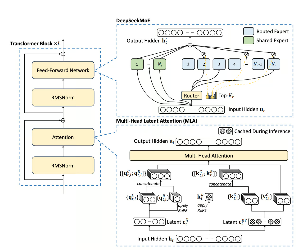
Image source
In this post, we will cover the main architectural aspects of the DeepSeek-V3-Base Technical Report, which describes the base model that is later used to train R1-Zero and R1 using GRPO.
For now, we will concentrate on the architectural innovations that DeepSeek achieved in their MoE base model, which we can summarize in three steps:
- DeepSeekMoE: Introducing a new approach for the Mixture of Experts model in conjunction with a method for Auxiliary-Loss-Free Load Balancing.
- MLA (Multi-Head Latent Attention): A nearly loss-free alternative to GQA.
- Multi Token Prediction: Enhancing training efficiency by predicting multiple tokens simultaneously.
Prerequisites
To understand the innovations in the MoE setting and Multi-Head Latent Attention (MLA), we will quickly (re)introduce both of them.
Mixture of Experts (MoE)
In our standard transformer block, recall that the FFN layer follows the RMSNorm of the MHA layer. The MoE architecture—which gained wide popularity after its use in GShard—replaces precisely this layer in a decoder block. The overall idea is to replace the large FFN with multiple smaller FFNs, called experts, each of which processes tokens based on a learned probability distribution. The network that generates this distribution is known as the router.
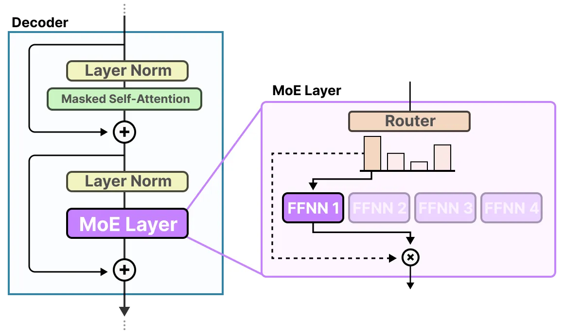
Image source
Mathematically, this can be expressed as follows:
Let and denote the sequence length and hidden dimension, respectively.
We consider a set of experts and
a gating (routing) function .
Then, for each token embedding ,
the output of the Mixture of Experts layer is computed as a weighted sum of the expert outputs:
Aggregating over the sequence, we obtain
where denotes the gating weight corresponding to expert , with . The reason this architecture has gained so much traction is that if is sparse, only a small subset of experts will ever be active at once. Consequently, we can scale the parameter count to trillions while only activating a small subset at any given time, thereby reducing memory requirements. This approach leverages the network’s ability to learn which subset of experts to use in a given context without having to evaluate a massive dense network.
In practice, our gating function is also modeled via an FFN.
Top-K Sampling
To make the vector sparse, both GShard and Switch Transformer have popularized the method of top- sampling. Instead of summing over all the weighted expert outputs, we only keep the highest values for any given and disregard the values of the other experts. Switch Transformer pushed this to its limits by setting , which was previously thought to be infeasible. Mathematically we can overall express this as:
where is the final output of the decoder block and implements the gating network, which is often just a simple perceptron.
Auxiliary Loss & Expert Capacity
When training such MoE models, as described above, we often encounter several issues. One common problem is the over-utilization of one or just a few experts. For example, due to chance during the early stages of training, one expert might yield a slightly lower loss, which causes the gating network to over-rely on that expert. This imbalance means that the other experts receive little to no training, reinforcing the problem and leading to suboptimal overall performance.
The solution to this issue is the introduction of an additional loss term called the auxiliary loss. This loss is used to encourage the network to evenly distribute its selections across all experts during training. We define this loss as:
where is the fraction of tokens routed to expert , which the model can influence by adjusting , the empirical average probability of a token being routed to expert . The scaling factor is introduced as a hyper-parameter. To prevent a single expert from being overloaded, we define an additional hard limit on how many tokens an expert can handle per batch. This limit is called the expert capacity. While the exact definition may vary from paper to paper, the one introduced in Switch Transformer is defined as:
While tokens that exceed the capacity limit are often dropped—meaning their computation is skipped and they are passed to a later layer via the skip connection, later methods have experimented with dynamically redistributing those tokens to underutilized experts. Again we introduce the capacity factor as a hyper-parameter.
DeepSeek-V3-Base Architecture
Now that we have covered the required prerequisites, let's take a closer look at the overall architecture of DeepSeek-V3. We'll begin with the new MoE layer, DeepSeekMoE, which was introduced in our previous paper.
DeepSeekMoE
DeepSeekMoE introduces several changes to the standard MoE architecture. One key innovation is what we call Fine-Grained Expert Segmentation. In this approach, the number of experts is increased by a factor of , while the hidden dimension of each expert is scaled down by a factor of . As a result, the top- selection is adjusted to a new value of .
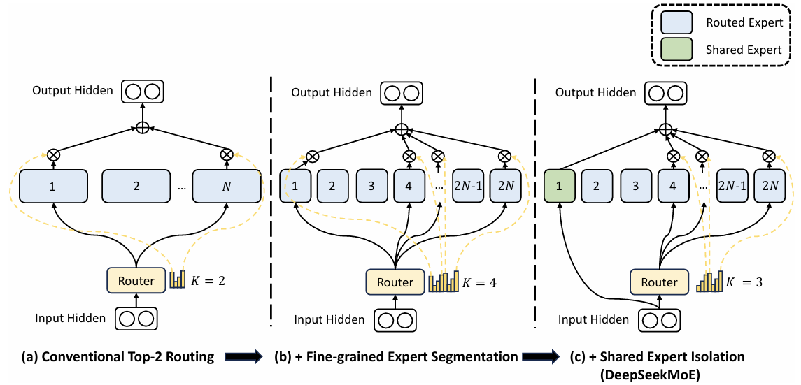
Image source
As illustrated above (in part (b)), when we set and hence (for example, if then ), the rationale is to increase the combinatorial complexity of the activated experts. For instance, with experts and a top-2 routing strategy, there are
different combinations of experts. However, if we set , then the effective number of experts becomes , and with a top routing value of , we obtain
different combinations of active experts—all while keeping the overall parameter count roughly the same.
Additionally, DeepSeekMoE introduces the concept of shared experts (part (c)). The idea is that each expert may need to learn some common knowledge, and if each expert learns it individually, it leads to a lot of redundancy in their parameters. To model this shared information more efficiently, we introduce a set of shared experts whose goal is to capture this common knowledge. This increases parameter efficiency for the remaining experts. For this to work properly, the shared experts are excluded from the routing mechanism so that every token passes through every shared expert.Given that denotes the number of shared experts and the number of routed experts, DeepSeek-V3 expresses it's MoE layer as follows:
where is a weight vector. Lastly, DeepSeek‑V3 introduces an auxiliary-loss-free load balancing method that ensures an even distribution of expert utilization without adding a separate loss term. In this approach, an additional bias is incorporated into the formulation of :
The bias is then dynamically adjusted during training: it is decreased by if expert is considered overloaded and increased by if it is underloaded. Although the paper does not explicitly specify the criteria for these states, they are likely determined relative to the balanced load, which can be estimated as (with being the total number of tokens). Although we overall refer to this MoE model as auxiliary-loss-free, the authors introduce an additional loss term, called the Complementary Sequence-Wise Auxiliary Loss, which enforces a balanced expert load within each sequence. This is particularly beneficial during inference, as it helps ensure that the experts, and consequently the GPU resources, are evenly distributed.
where is the number of tokens in the sequence. We can see that represents the fraction of tokens in the sequence routed to expert , scaled by the ratio of the total number of routed experts to the number of active experts. This is then weighted by the average probability that an expert is chosen within the sequence and summed over all routed experts. Note that this formulation of the loss is essentially the same as the auxiliary loss, but it uses empirical averages over intra-sequence statistics. To ensure that the influence of this term remains rather small, leaving most of the load balancing work to the bias term, we set
KV-Caching
As a refresher we will quickly again cover Key-Value-Caching, which we already covered in a previous post.
One of the most important optimizations that Llama has introduced in their architecture is the so-called key-value cache. The purpose of this becomes clear if we look at the figure below:
Image source
As you know, during inference we sample the next token and append it to the sequence before we feed this new sequence into the transformer to predict the next token. But as you can see in the figure, to predict token 5, we only need query token 4 to multiply with the keys. This means to predict token 5, we only need the last row of the attention matrix. Thus, instead of feeding in the entire sequence of tokens of length to predict , we just feed in the -th token. For the attention and subsequent multiplication with , however, we still need the previous tokens. This is exactly where the key-value cache (kv-cache) comes in.
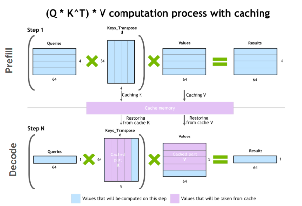
Image source
For every token we see, we save it in the kv-cache for later usage in the multiplications. By doing this, we can save a significant amount of attention multiplications, as we only need to compute the last row of the attention matrix! Nice!
Multi-Head Latent Attention (MLA)
Multi-Head Latent Attention was first introduced by DeepSeek-V2 and is a revolutionary approach to drastically reducing the size of the KV-cache during inference. Let's, for example, consider the architecture of DeepSeek-V3 and calculate its memory requirements during inference when using its 100K token context window.
For DeepSeek-V3, we have a head dimension of , with heads per attention layer. In total, there are such layers. If we now use FP16 precision for each weight and our full context window , we arrive at a KV-cache size of
This means the size of our KV-cache for a full context window is approximately 400GB! This is tremendous, and therefore there have been multiple suggestions over the years to save space in the KV-cache. One of these, which found application in the architecture of Llama3, is GQA (Grouped Query Attention), where multiple query heads share a single key and value head, although this comes at the cost of accuracy.
The idea of MLA is now to compress our incoming token embedding , where is the sequence length and is the embedding dimension, with a learned weight matrix , to obtain
where and is the compressed latent representation of keys and values of token . To obtain our keys and values, we define and which will learn to upscale our compressed representation
After this, we resume with our standard attention mechanism. Now, before covering the genius of this approach, note that through this low‐rank approximation of the traditional via , we achieve a smaller parameter count because . This is very similar to what we do when fine-tuning with LoRA to minimize the number of parameters we have to tune.
One might be tempted to think that we have just traded reduced memory requirements for increased computational demand by introducing two new matrices. However, this is exactly where the ingenuity of MLA lies. We only have to learn and store the additional matrices and during training. During inference, however, where the KV-cache normally comes into play, we are able to precompute and . As the following relations hold
From this, we can conclude that the standard attention mechanism will look like
We can rewrite this by regrouping terms of and , resulting in
As we can see, during inference we can precompute for every layer and use the cached for the attention calculation, thereby not incurring any additional computational cost with this approach.
Similarly, we can precompute In multi-head attention, we combine the results from all heads and project them using :
Using associativity, we finally end up with
However, DeepSeek-V3-Base introduces an additional step for the Rotary Positional Embedding.
The complete MLA formulation from the paper is given as
It is important to note that denotes the index of the t-th token and the number of attention heads.
As we can see, the formulation introduces an additional term , which carries the positional information of the token at position .
Here, is a projection matrix, where specifies the number of dimensions used to down-project before applying the Rotary Positional Embedding (RoPE).
Finally, we concatenate and to form the complete key vector for token and attention head . During inference, we only need to store and , both of which are significantly smaller than storing the full key and value vectors for each token at their original embedding dimension.
Additionally they introduce a low-rank compressiion for the queries, which are not stored as the ones for keys and values, but are soley used due to their lower activation memory during training and inference.
Again, we introduce a down-projection matrix ,
where, as before, .
When we need again, we can recompute it via , with .
They further use to encode the compressed latent representation using RoPE, and finally concatenate both and to obtain the complete query vector for token and head
This way, we do not need to store during training but can simply recompute it during the backward pass, thereby saving precious GPU memory.
Multi-Token Prediction
Another important step in the training of DeepSeek-V3-Base was the introduction of MTP. Instead of calculating the loss solely by aggregating the CrossEntropy between the predicted token distribution and the ground truth, the model is additionally forced to predict the k-th subsequent tokens. The authors justify this approach by arguing that it may both densify the training signal and help the model better plan the prediction of future tokens.
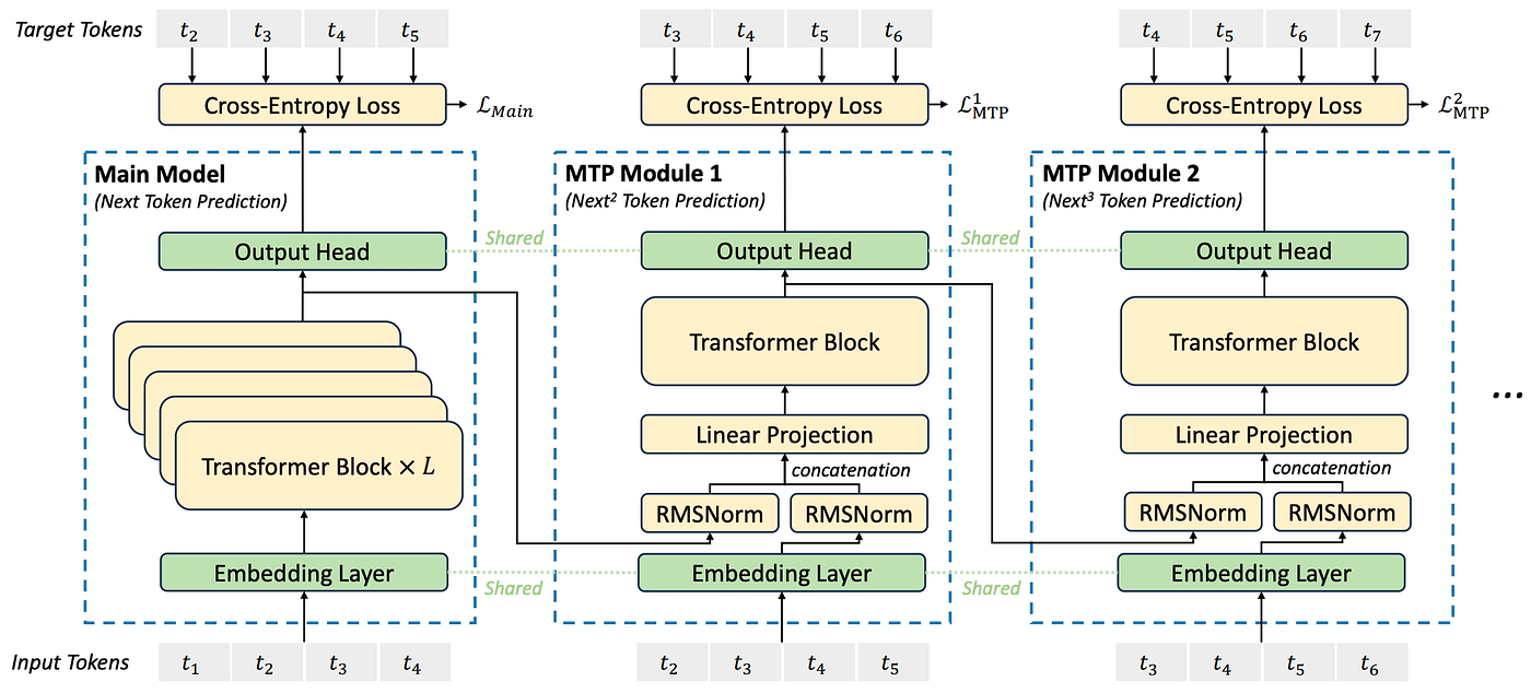
Image source
Each subsequent token is predicted using an MTP block (see Eq.). These blocks consist of a shared embedding layer and output head from the main model, together with a Transformer block () and a linear projection matrix . As shown in the figure, we take the output of the -th token from the -th MTP block and normalize it using . In addition, we compute the embedding of the -th token using the shared embedding layer. Both representations are then concatenated and projected through , yielding
We now use the representations as inputs to the Transformer block:
Note that we only use the original input tokens within the Transformer. As illustrated in the figure, the embeddings of future tokens are computed and incorporated during the concatenation and projection step; however, the Transformer itself operates solely on .
The output of the Transformer block, , is then fed into the shared output head to predict the probability distribution for the token :
For the loss calculation, we use the following setup. Recall that for the first MTP block (), we aim to predict the token . Therefore, for the first input token , the prediction target becomes . Accordingly, the loss formulation for an MTP module is given by
Finally, we average these losses over all prediction depths and weight them by a scaling factor :
Note that this entire multi-token prediction procedure is applied solely during training to enhance the model's ability to anticipate future tokens. During inference, the MTP blocks are not used.